🟢 pp2 example from AUTO07p (aBD + Hopf aBS)

The goal of this example is to show how to use automatic bifurcation diagram computation for a simple ODE.

The following equations are a model of type predator-prey. The example is taken from Auto07p:

\[\begin{array}{l} u_{1}^{\prime}=3 u_{1}\left(1-u_{1}\right)-u_{1} u_{2}-p_1\left(1-e^{-5 u_{1}}\right) \\ u_{2}^{\prime}=-u_{2}+3 u_{1} u_{2} \end{array}\]

It is easy to encode the ODE as follows

using Revise, Plotsimport BifurcationKit as BKimport BifurcationKit: @optic#, @reset# function to record information from a solutionrecordFromSolution(x, p; k...) = (u1 = x[1], u2 = x[2])function pp2!(dz, z, p, t = 0)	(;p1, p2, p3, p4) = p	u1, u2 = z	dz[1] = p2 * u1 * (1 - u1) - u1 * u2 - p1 * (1 - exp(-p3 * u1))	dz[2] =	-u2 + p4 * u1 * u2	dzend# parameters of the modelpar_pp2 = (p1 = 1., p2 = 3., p3 = 5., p4 = 3.)# initial conditionz0 = zeros(2)# bifurcation problemprob = BK.ODEBifProblem(pp2!, z0, par_pp2,	# specify the continuation parameter	(@optic _.p1), record_from_solution = recordFromSolution)

Automatic bifurcation diagram computation

We set up the options or the continuation

# continuation optionsopts_br = BK.ContinuationPar(p_min = 0.1, p_max = 1.0, dsmax = 0.01,	# maximum number of continuation steps	max_steps = 1000,)

ContinuationPar{Float64, DefaultLS, DefaultEig{typeof(real)}}
    ┌─ a = 0.5
    ├─ detect_bifurcation = 3
    ├─ detect_event = 0
    ├─ detect_fold = true
    ├─ detect_loop = false
    ├─ ds = 0.01
    ├─ dsmax = 0.01
    ├─ dsmin = 0.0001
    ├─ dsmin_bisection = 1.0e-16
    ├─ max_bisection_steps = 25
    ├─ max_steps = 1000
    ├─ n_inversion = 2
    ├─ nev = 3
    ├─ newton_options = NewtonPar{Float64, DefaultLS, DefaultEig{typeof(real)}}
    ├─ p_max = 1.0
    ├─ p_min = 0.1
    ├─ plot_every_step = 10
    ├─ save_eig_every_step = 1
    ├─ save_eigenvectors = true
    ├─ save_sol_every_step = 1
    ├─ save_to_file = false
    ├─ tol_bisection_eigenvalue = 1.0e-16
    ├─ tol_param_bisection_event = 1.0e-16
    ├─ tol_stability = 1.0e-10
    └─ η = 150.0

We are now ready to compute the diagram

diagram = BK.bifurcationdiagram(prob, BK.PALC(),	# very important parameter. It specifies the maximum amount of recursion	# when computing the bifurcation diagram. It means we allow computing branches of branches of branches	# at most in the present case.	3,	BK.ContinuationPar(opts_br; ds = -0.001, dsmax = 0.01, n_inversion = 8, detect_bifurcation = 3),	)scene = plot(diagram; code = (), title="$(size(diagram)) branches", legend = false)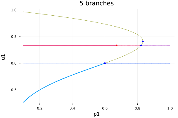

Branch of periodic orbits with collocation method

As you can see on the diagram, there is a Hopf bifurcation indicated by a red dot. Let us compute the periodic orbit branching from the Hopf point.

We first find the branch

# branch of the diagram with Hopf pointbrH = BK.get_branch(diagram, (2,2)).γ# continuation parametersopts_po_cont = BK.ContinuationPar(dsmax = 0.01, ds= 0.0001, dsmin = 1e-4,	tol_stability = 1e-4, max_steps = 100, detect_bifurcation = 2)br_po = BK.continuation(	brH, 1, opts_po_cont,	BK.Collocation(20, 5);	normC = BK.norminf)plot(diagram); plot!(br_po, branchlabel = "Periodic orbits", legend = :bottomright)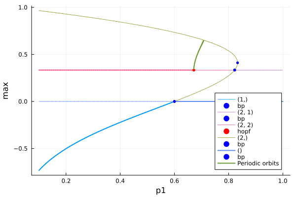

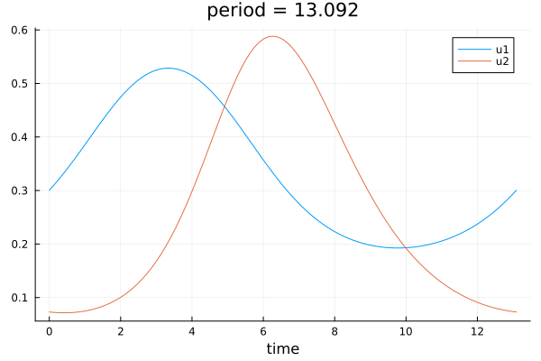
Let us now plot an orbit

# extract the different componentsorbit = BK.get_periodic_orbit(br_po, 30)plot(orbit.t, orbit[1,:]; label = "u1", markersize = 2)plot!(orbit.t, orbit[2,:]; label = "u2", xlabel = "time", title = "period = $(round(orbit.t[end], digits = 3))")