Interpolation using different methods

We will use the following data to demonstrate interpolation methods.

using DataInterpolations, Plots

# Dependent variable
u = [14.7, 11.51, 10.41, 14.95, 12.24, 11.22]

# Independent variable
t = [0.0, 62.25, 109.66, 162.66, 205.8, 252.3]

6-element Vector{Float64}:
   0.0
  62.25
 109.66
 162.66
 205.8
 252.3

For each method, we will show how to perform the fit and use the plot recipe to show the fitting curve.

Linear Interpolation

This is a linear interpolation between the ends points of the interval of input data points.

A = LinearInterpolation(u, t)
plot(A)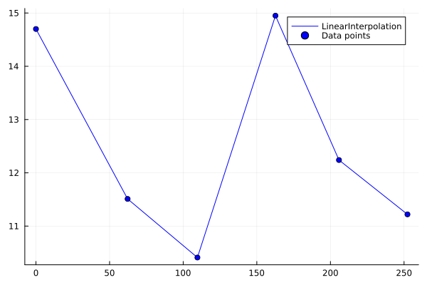

Quadratic Interpolation

This function fits a parabola passing through the two nearest points from the input data point as well as the next-closest point on the right or left, depending on whether the forward- or backward-looking mode is selected (default mode is forward-looking). It is continuous and piecewise differentiable.

A = QuadraticInterpolation(u, t) # same as QuadraticInterpolation(u,t,:Forward)
# alternatively: A = QuadraticInterpolation(u,t,:Backward)
plot(A)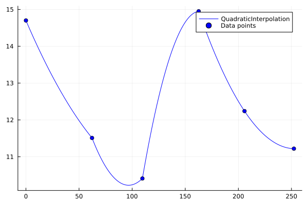

Lagrange Interpolation

It fits a polynomial of degree d (=length(t)-1), and is thus a continuously differentiable function.

A = LagrangeInterpolation(u, t)
plot(A)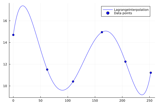

Akima Interpolation

This function fits piecewise cubic polynomials which forms a continuously differentiable function. This differs from Cubic Spline as coefficients are computed using only neighbouring points and hence the fit looks more natural.

A = AkimaInterpolation(u, t)
plot(A)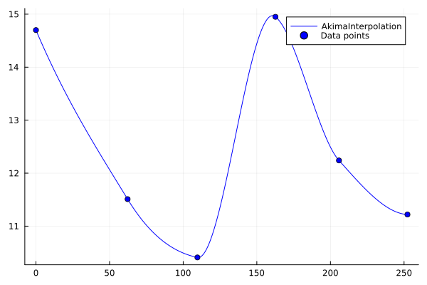

Constant Interpolation

This function is constant between data points. By default, it takes the value at the left end of the interval. One can change that behavior by passing the keyword argument dir = :right.

A = ConstantInterpolation(u, t)
plot(A)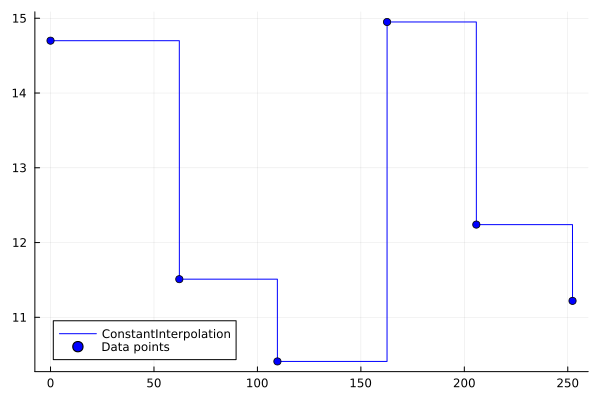

Or using the right endpoints:

A = ConstantInterpolation(u, t, dir = :right)
plot(A)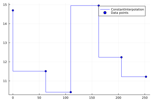

Smoothed Constant Interpolation

This function is much like the constant interpolation above, but the transition between consecutive values is smoothed out so that the function is continuously differentiable. The smoothing is done in such a way that the integral of this function is never much off from the same integral of constant interpolation without smoothing (because of the symmetry of the smoothing sections). The maximum smoothing distance in the t direction from the data points can be set with the keyword argument d_max.

A = ConstantInterpolation(u, t)
plot(A)
A = SmoothedConstantInterpolation(u, t; d_max = 10)
plot!(A)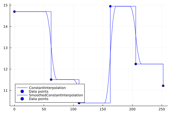

Note that u[end] is ignored, except when using extrapolation types Constant or Extension.

Quadratic Spline

This is the quadratic spline. It is a continuously differentiable interpolation which hits each of the data points exactly. Unlike a piecewise polynomial built directly from the data (e.g. Quadratic Interpolation), the control points of a quadratic spline are solved for globally to satisfy continuity of the derivative at every knot, so changing a single data point can, in principle, affect the curve everywhere rather than only near that point.

A = QuadraticSpline(u, t)
plot(A)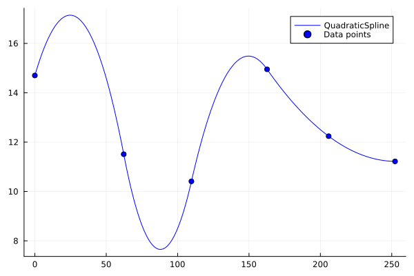

Cubic Spline

This is the cubic spline. It is a continuously twice differentiable interpolation which hits each of the data points exactly. As with Quadratic Spline, its control points are solved for globally, so changing a single data point can, in principle, affect the curve everywhere rather than only near that point.

A = CubicSpline(u, t)
plot(A)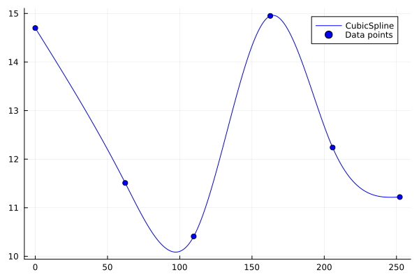

B-Splines

This is an interpolating B-spline. B-splines are a global method, meaning that every data point is taken into account for each point of the curve. The interpolating B-spline is the version which hits each of the points. This method is described in more detail here. Let's plot a cubic B-spline (3rd order). Since the data points are not close to uniformly spaced, we will use the :Average knot vector:

A = BSplineInterpolation(u, t, 3, :Average)
plot(A)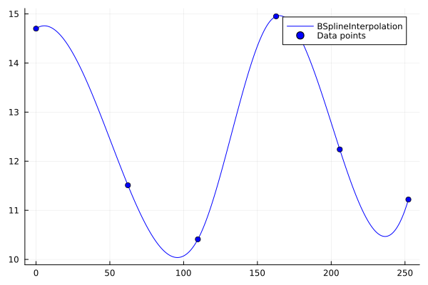

The approximating B-spline is a smoothed version of the B-spline. It again is a global method. In this case, we need to give a number of control points length(t)>h and this method fits a B-spline through the control points which is a least square approximation. This has a natural effect of smoothing the data. For example, if we use 4 control points, we get the result:

A = BSplineApprox(u, t, 3, 4, :Average)
plot(A)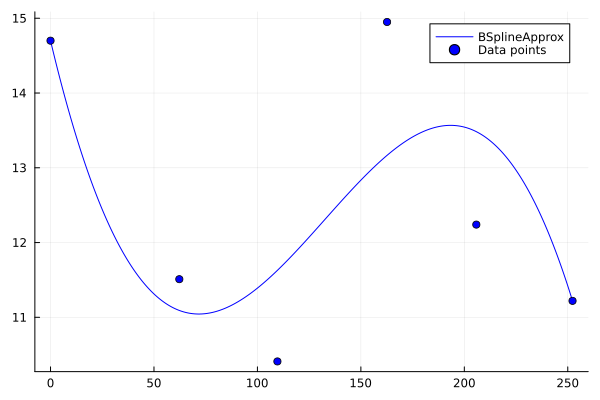

Cubic Hermite Spline

This is the cubic (third order) Hermite interpolation. It matches the values and first order derivatives in the data points exactly.

du = [-0.047, -0.058, 0.054, 0.012, -0.068, 0.0011]
A = CubicHermiteSpline(du, u, t)
plot(A)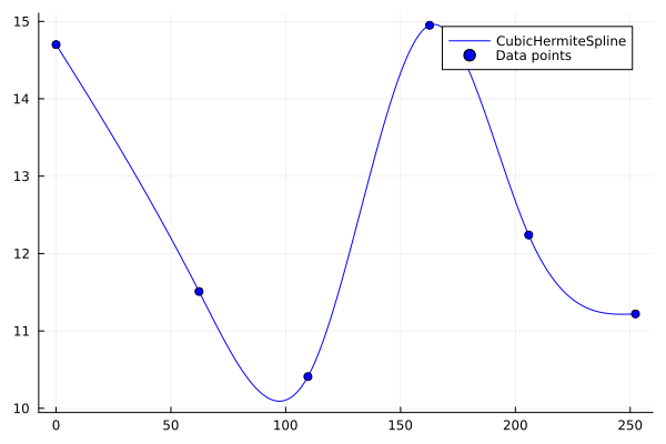

PCHIP Interpolation

This is a type of CubicHermiteSpline where the derivative values du are derived from the input data in such a way that the interpolation never overshoots the data.

A = PCHIPInterpolation(u, t)
plot(A)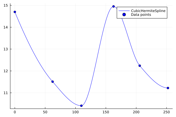

Quintic Hermite Spline

This is the quintic (fifth order) Hermite interpolation. It matches the values and first and second order derivatives in the data points exactly.

ddu = [0.0, -0.00033, 0.0051, -0.0067, 0.0029, 0.0]
du = [-0.047, -0.058, 0.054, 0.012, -0.068, 0.0011]
A = QuinticHermiteSpline(ddu, du, u, t)
plot(A)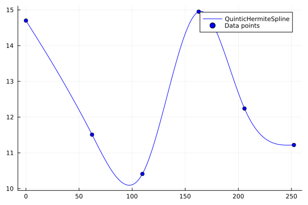

Dense Data Demonstration

Some methods are better suited for dense data. Let's generate such data to demonstrate these methods.

import StableRNGs: StableRNG
rng = StableRNG(318)
t = sort(10 .* rand(rng, 100))
u = sin.(t) .+ 0.5 * randn(rng, 100);

100-element Vector{Float64}:
 -0.4891563556934994
 -0.7411337336203204
  0.303260759772529
 -0.03721116720925663
 -0.5073147206014983
  0.1956851914978695
  0.5717256362165741
  0.29209309353794644
  0.6444380583968424
  0.5907863715716408
  ⋮
  1.4566016140618308
  1.016810621114802
  0.32542000692979595
  1.1323247210598848
 -0.0495435623347093
  0.1762559989623056
 -0.5319640155153034
 -0.9932887141154423
 -1.2766512199488596

Curve Fits

A curve fit works with both dense and sparse data. We will demonstrate the curve fit on the dense data since we generated it based on sin(t), so this is the curve we want to fit through it. To do so, let's define a similar function with parameters. Let's choose the form:

m(t, p) = @. p[1] * sin(p[2] * t) + p[3] * cos(p[4] * t)

m (generic function with 1 method)

Notice that this is a function on the whole array of t and expects an array for the predicted u out. This choice of m is based on the assumption that our function is of the form p1*sin(p2*t)+p3*cos(p4*t). We want to find the p to match our data. Let's start with the guess of every p being zero, that is p=ones(4). Then we would fit this curve using:

using CurveFit
A = Curvefit(u, t, m, ones(4))
plot(A)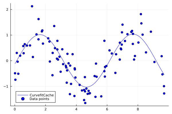

We can check what the fitted parameters are via:

A.pmin

4-element Vector{Float64}:
  1.0025173183429874
  1.0396588439617964
 -0.13178842437438515
  1.0670107403746447

Notice that it essentially made p3=0 with p1=p2=1, meaning it approximately found sin(t)! But note that the ability to fit is dependent on the initial parameters. For example, with p=zeros(4) as the initial parameters, the fit is not good:

A = Curvefit(u, t, m, zeros(4))
plot(A)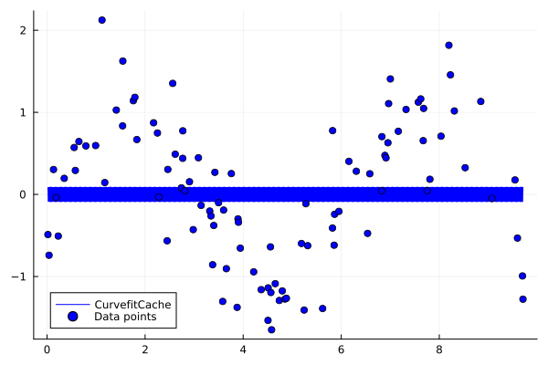

And the parameters show the issue:

A.pmin

4-element Vector{Float64}:
   0.0
   0.0
   0.08737216770173488
 642.2388327736436

Curvefit(
        u, t, model, p0, alg, box = false, lb = nothing, ub = nothing;
        extrapolate = false
    ) -> CurvefitCache

using DataInterpolations, Optim

model(t, p) = p[1] .* t .+ p[2]
A = Curvefit([1.0, 3.0, 5.0], [0.0, 1.0, 2.0], model, [0.0, 0.0], LBFGS())

A(1.5)