Multiple Shooting

In Multiple Shooting, the training data is split into overlapping intervals. The solver is then trained on individual intervals. If the end conditions of any interval coincide with the initial conditions of the next immediate interval, then the joined/combined solution is the same as solving on the whole dataset (without splitting).

To ensure that the overlapping part of two consecutive intervals coincide, we add a penalizing term:

continuity_term * absolute_value_of(prediction of last point of group i - prediction of first point of group i+1)

to the loss.

Note that the continuity_term should have a large positive value to add high penalties in case the solver predicts discontinuous values.

The following is a working demo, using Multiple Shooting:

using ComponentArrays,
    Lux, DiffEqFlux, Optimization, OptimizationPolyalgorithms, OrdinaryDiffEq, Plots
using DiffEqFlux: group_ranges

using Random
rng = Random.default_rng()

# Define initial conditions and time steps
datasize = 30
u0 = Float32[2.0, 0.0]
tspan = (0.0f0, 5.0f0)
tsteps = range(tspan[1], tspan[2]; length = datasize)

# Get the data
function trueODEfunc(du, u, p, t)
    true_A = [-0.1 2.0; -2.0 -0.1]
    du .= ((u .^ 3)'true_A)'
end
prob_trueode = ODEProblem(trueODEfunc, u0, tspan)
ode_data = Array(solve(prob_trueode, Tsit5(); saveat = tsteps))

# Define the Neural Network
nn = Chain(x -> x .^ 3, Dense(2, 16, tanh), Dense(16, 2))
p_init, st = Lux.setup(rng, nn)

neuralode = NeuralODE(nn, tspan, Tsit5(); saveat = tsteps)
prob_node = ODEProblem((u, p, t) -> nn(u, p, st)[1], u0, tspan, ComponentArray(p_init))

function plot_multiple_shoot(plt, preds, group_size)
    step = group_size - 1
    ranges = group_ranges(datasize, group_size)

    for (i, rg) in enumerate(ranges)
        plot!(plt, tsteps[rg], preds[i][1, :]; markershape = :circle, label = "Group $(i)")
    end
end

anim = Plots.Animation()
iter = 0
callback = function (p, l, preds; doplot = true)
    display(l)
    global iter
    iter += 1
    if doplot && iter % 1 == 0
        # plot the original data
        plt = scatter(tsteps, ode_data[1, :]; label = "Data")

        # plot the different predictions for individual shoot
        plot_multiple_shoot(plt, preds, group_size)

        frame(anim)
        display(plot(plt))
    end
    return false
end

# Define parameters for Multiple Shooting
group_size = 3
continuity_term = 200

function loss_function(data, pred)
    return sum(abs2, data - pred)
end

ps = ComponentArray(p_init)
pd, pax = getdata(ps), getaxes(ps)

function loss_multiple_shooting(p)
    ps = ComponentArray(p, pax)
    return multiple_shoot(ps, ode_data, tsteps, prob_node, loss_function, Tsit5(),
        group_size; continuity_term)
end

adtype = Optimization.AutoZygote()
optf = Optimization.OptimizationFunction((x, p) -> loss_multiple_shooting(x), adtype)
optprob = Optimization.OptimizationProblem(optf, pd)
res_ms = Optimization.solve(optprob, PolyOpt(); callback = callback)
gif(anim, "multiple_shooting.gif"; fps = 15)

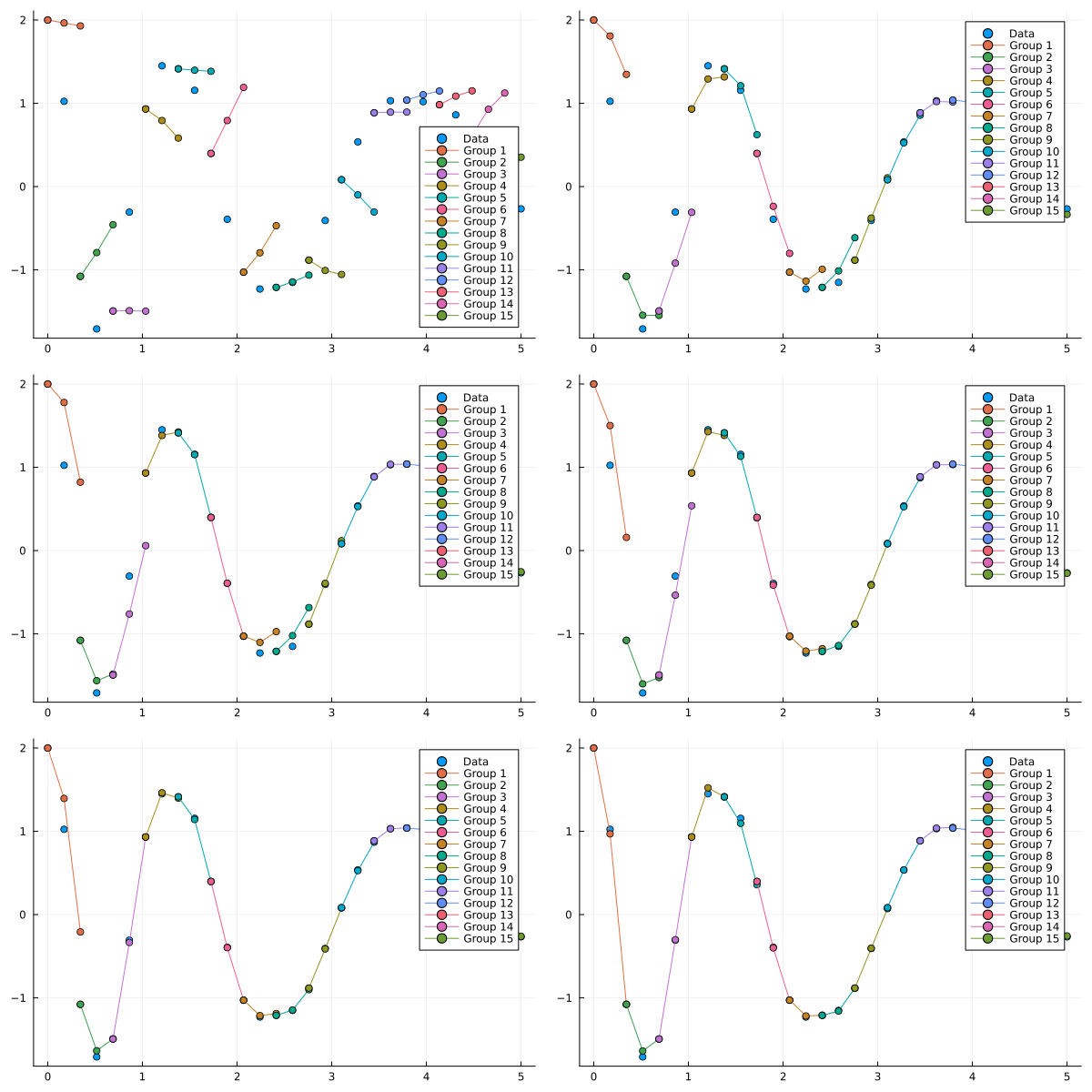
The connected lines show the predictions of each group. Notice that there are overlapping points as well. These are the points we are trying to coincide.

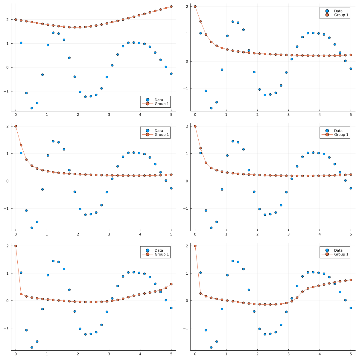
Here is an output with group_size = 30 (which is the same as solving on the whole interval without splitting also called single shooting).

anim = Plots.Animation()
iter = 0
group_size = 30

ps = ComponentArray(p_init)
pd, pax = getdata(ps), getaxes(ps)

function loss_single_shooting(p)
    ps = ComponentArray(p, pax)
    return multiple_shoot(ps, ode_data, tsteps, prob_node, loss_function, Tsit5(),
        group_size; continuity_term)
end

adtype = Optimization.AutoZygote()
optf = Optimization.OptimizationFunction((x, p) -> loss_single_shooting(x), adtype)
optprob = Optimization.OptimizationProblem(optf, pd)
res_ms = Optimization.solve(optprob, PolyOpt(); callback = callback)
gif(anim, "single_shooting.gif"; fps = 15)

It is clear from the above picture, a single shoot doesn't perform very well with the ODE Problem we have and gets stuck in a local minimum.