Noise Processes API
Core Types
DiffEqNoiseProcess.NoiseProcess — Type
NoiseProcess{T, N, Tt, T2, T3, ZType, F, F2, inplace, S1, S2, RSWM, C, RNGType} <:
{T, N, Vector{T2}, inplace}
A NoiseProcess is a type defined as:
NoiseProcess(t0, W0, Z0, dist, bridge;
    iip = SciMLBase.isinplace(dist, 3),
    rswm = RSWM(), save_everystep = true,
    rng = Random.default_rng(),
reset = true, reseed = true)t0is the first timepointW0is the first value of the process.Z0is the first value of the pseudo-process. This is necessary for higher order algorithms. If it's not needed, set tonothing.distthe distribution of the steps over time.bridgethe bridging distribution. Optional, but required for adaptivity and interpolating at new values.covarianceis the covariance matrix of the noise process. If not provided, the noise is assumed to be uncorrelated in each variable.save_everystepwhether to save every step of the Brownian timeseries.rngthe local RNG used for generating the random numbers.resetwhether to reset the process with each solve.reseedwhether to reseed the process with each solve.
Fields
t: Saved time points, in traversal order.W: Saved primary process values corresponding tot.Z: Saved auxiliary process values, ornothingwhen unused.curt,curW,curZ: Current time and current primary/auxiliary values.dt,dW,dZ: Proposed step width and pending increments.dist,bridge: Step and bridge callbacks.covariance,rswm,save_everystep,rng,reset,reseed,continuous: Process configuration.
The stack and scratch-buffer fields are implementation details. Solvers should use the exported step functions instead of reading or mutating those fields.
The signature for the dist is:
dist!(rand_vec, dW, W, dt, u, p, t, rng)for inplace functions, and:
rand_vec = dist(dW, W, dt, u, p, t, rng)otherwise. The signature for bridge is:
bridge!(rand_vec, dW, W, W0, Wh, q, h, u, p, t, rng)and the out of place syntax is:
rand_vec = bridge(dW, W, W0, Wh, q, h, u, p, t, rng)Here, W is the noise process, W0 is the left side of the current interval, Wh is the right side of the current interval, h is the interval length, and q is the proportion from the left where the interpolation is occurring.
Direct Construction Example
The easiest way to show how to directly construct a NoiseProcess is by example. Here we will show how to directly construct a NoiseProcess which generates Gaussian white noise.
This is the noise process, that uses randn!. A special dispatch is added for complex numbers for (randn()+im*randn())/sqrt(2). This function is DiffEqNoiseProcess.wiener_randn (or with ! respectively).
The first function that must be defined is the noise distribution. This is how to generate $W(t+dt)$ given that we know $W(x)$ for $x∈[t₀,t]$. For Gaussian white noise, we know that
\[W(dt) ∼ N(0,dt)\]
for $W(0)=0$ which defines the stepping distribution. Thus, its noise distribution function is:
@inline function WHITE_NOISE_DIST(dW, W, dt, u, p, t, rng)
    if W.dW isa AbstractArray && !(W.dW isa SArray)
        return @fastmath sqrt(abs(dt)) * wiener_randn(rng, W.dW)
    else
        return @fastmath sqrt(abs(dt)) * wiener_randn(rng, typeof(W.dW))
    end
end
for the out of place versions, and for the inplace versions
function INPLACE_WHITE_NOISE_DIST(rand_vec, dW, W, dt, u, p, t, rng)
    wiener_randn!(rng, rand_vec)
    sqrtabsdt = @fastmath sqrt(abs(dt))
    @. rand_vec *= sqrtabsdt
end
Optionally, we can provide a bridging distribution. This is the distribution of $W(qh)$ for $q∈[0,1]$ given that we know $W(0)=0$ and $W(h)=Wₕ$. For Brownian motion, this is known as the Brownian Bridge, and is well known to have the distribution:
\[W(qh) ∼ N(qWₕ,(1-q)qh)\]
Thus, we have the out-of-place and in-place versions as:
function WHITE_NOISE_BRIDGE(dW, W, W0, Wh, q, h, u, p, t, rng)
    if W.dW isa AbstractArray
        return @fastmath sqrt((1 - q) * q * abs(h)) * wiener_randn(rng, W.dW) + q * Wh
    else
        return @fastmath sqrt((1 - q) * q * abs(h)) * wiener_randn(rng, typeof(W.dW)) +
                         q * Wh
    end
end
function INPLACE_WHITE_NOISE_BRIDGE(rand_vec, dW, W, W0, Wh, q, h, u, p, t, rng)
    wiener_randn!(rng, rand_vec)
    #rand_vec .= sqrt((1.-q).*q.*abs(h)).*rand_vec.+q.*Wh
    sqrtcoeff = @fastmath sqrt((1 - q) * q * abs(h))
    @. rand_vec = sqrtcoeff * rand_vec + q * Wh
end
These functions are then placed in a noise process:
NoiseProcess(t0, W0, Z0, WHITE_NOISE_DIST, WHITE_NOISE_BRIDGE; kwargs)
NoiseProcess(t0, W0, Z0, INPLACE_WHITE_NOISE_DIST, INPLACE_WHITE_NOISE_BRIDGE; kwargs)
Notice that we can optionally provide an alternative adaptive algorithm for the timestepping rejections. RSWM() defaults to the Rejection Sampling with Memory 3 algorithm (RSwM3).
Note that the standard constructors are simply:
function WienerProcess(t0, W0, Z0 = nothing)
    NoiseProcess(t0, W0, Z0, WHITE_NOISE_DIST, WHITE_NOISE_BRIDGE; kwargs)
end
function WienerProcess!(t0, W0, Z0 = nothing)
    NoiseProcess(t0, W0, Z0, INPLACE_WHITE_NOISE_DIST, INPLACE_WHITE_NOISE_BRIDGE; kwargs)
end
These will generate a Wiener process, which can be stepped with step!(W,dt), and interpolated as W(t).
DiffEqNoiseProcess.SimpleNoiseProcess — Type
SimpleNoiseProcess{T, N, Tt, T2, T3, ZType, F, F2, inplace, RNGType} <:
AbstractNoiseProcess{T, N, Vector{T2}, inplace}
Like NoiseProcess but without support for adaptivity. This makes it lightweight and slightly faster.
SimpleNoiseProcess should not be used with adaptive SDE solvers as it will lead to incorrect results.
SimpleNoiseProcess{iip}(t0, W0, Z0, dist, bridge;
    save_everystep = true,
    rng = Random.default_rng(),
reset = true, reseed = true) where {iip}t0is the first timepointW0is the first value of the process.Z0is the first value of the pseudo-process. This is necessary for higher order algorithms. If it's not needed, set tonothing.distthe distribution for the steps over time.bridgethe bridging distribution. Optional, but required for adaptivity and interpolating at new values.save_everystepwhether to save every step of the Brownian timeseries.rngthe local RNG used for generating the random numbers.resetwhether to reset the process with each solve.reseedwhether to reseed the process with each solve.
Fields
t,W,Z: Saved times and primary/auxiliary values.curt,curW,curZ: Current time and current values.dt,dW,dZ: Proposed step and pending increments.dist,bridge: Distribution and bridge callbacks.covariance,save_everystep,rng,reset,reseed: Stored options.
The process does not retain rejection-memory stacks. Adaptive solvers must not call reject_step! on it.
Wiener Processes
Standard Wiener Process
DiffEqNoiseProcess.WienerProcess — Function
WienerProcess(t0, W0, Z0 = nothing; kwargs...)Construct an out-of-place Wiener process (Brownian motion). Its increments have distribution N(0, abs(dt)), and values between generated points are sampled with a Brownian bridge.
W = WienerProcess(0.0, 0.0)
sol = solve(NoiseProblem(W, (0.0, 1.0)); dt = 0.01)
sol(0.5)
Arguments
t0: Initial time.W0: Initial noise value and prototype for the process shape and element type.Z0: Optional auxiliary process value for higher-order methods.
Keywords
rswm: Rejection Sampling with Memory configuration.save_everystep: Whether to retain every generated time and value.covariance: Optional covariance metadata.rng: Random number generator used for increments.reset: Whether solving a problem reinitializes the process.reseed: Whether solving without an explicit seed reseedsrng.continuous: Whether interpolation includes the left endpoint in its mean.
Additional keywords are forwarded to NoiseProcess.
Returns
A NoiseProcess with isinplace(W) == false.
DiffEqNoiseProcess.WienerProcess! — Function
WienerProcess!(t0, W0, Z0 = nothing; kwargs...)Construct an in-place Wiener process. It has the same distribution and solver contract as WienerProcess, but its distribution and bridge functions write into preallocated storage.
W = WienerProcess!(0.0, zeros(2))
calculate_step!(W, 0.01, nothing, nothing)
Arguments
t0: Initial time.W0: Initial array-valued noise and storage prototype.Z0: Optional auxiliary process value.
Keywords
The same process-control keywords as WienerProcess are accepted and forwarded to NoiseProcess.
Returns
A NoiseProcess with isinplace(W) == true.
DiffEqNoiseProcess.SimpleWienerProcess — Function
SimpleWienerProcess(t0, W0, Z0 = nothing; kwargs...)Construct a lightweight out-of-place Wiener process. Unlike WienerProcess, this process cannot recover a rejected adaptive step and must be used with a fixed-step solver.
W = SimpleWienerProcess(0.0, 0.0)
sol = solve(NoiseProblem(W, (0.0, 1.0)); dt = 0.01)
Arguments
t0: Initial time.W0: Initial noise value and prototype for the process shape and element type.Z0: Optional auxiliary process value.
Keywords
save_everystep: Whether to retain every generated time and value.covariance: Optional covariance metadata.rng: Random number generator used for increments.reset: Whether solving a problem reinitializes the process.reseed: Whether solving without an explicit seed reseedsrng.
Additional keywords are forwarded to SimpleNoiseProcess.
Returns
A SimpleNoiseProcess with isinplace(W) == false.
DiffEqNoiseProcess.SimpleWienerProcess! — Function
SimpleWienerProcess!(t0, W0, Z0 = nothing; kwargs...)Construct an in-place lightweight Wiener process. It has the same non-adaptive restriction as SimpleWienerProcess.
W = SimpleWienerProcess!(0.0, zeros(2))
calculate_step!(W, 0.01, nothing, nothing)
Arguments
t0: Initial time.W0: Initial array-valued noise and storage prototype.Z0: Optional auxiliary process value.
Keywords
The same process-control keywords as SimpleWienerProcess are accepted and forwarded to SimpleNoiseProcess.
Returns
A SimpleNoiseProcess with isinplace(W) == true.
Real-Valued Wiener Process
DiffEqNoiseProcess.RealWienerProcess — Function
RealWienerProcess(t0, W0, Z0 = nothing; kwargs...)Construct an out-of-place Brownian process whose increments are real-valued, even when W0 is complex. This is useful for complex SDE states driven by real noise.
W = RealWienerProcess(0.0, 0.0 + 0im)Arguments
t0: Initial time.W0: Initial value and prototype for the process shape.Z0: Optional auxiliary process value.
Keywords
The same process-control keywords as WienerProcess are accepted.
Returns
A NoiseProcess with isinplace(W) == false.
DiffEqNoiseProcess.RealWienerProcess! — Function
RealWienerProcess!(t0, W0, Z0 = nothing; kwargs...)Construct the in-place variant of RealWienerProcess. It stores and updates its increment buffers rather than allocating new arrays.
W = RealWienerProcess!(0.0, zeros(2))
calculate_step!(W, 0.01, nothing, nothing)
Arguments
t0: Initial time.W0: Initial value and storage prototype.Z0: Optional auxiliary process value.
Keywords
The same process-control keywords as WienerProcess are accepted.
Returns
A NoiseProcess with isinplace(W) == true.
Correlated Wiener Process
DiffEqNoiseProcess.CorrelatedWienerProcess — Function
CorrelatedWienerProcess(Γ, t0, W0, Z0 = nothing; rng = Random.default_rng())Construct an out-of-place Wiener process with constant covariance matrix Γ. The covariance is factored once and applied to independent normal increments.
Γ = [1.0 0.2; 0.2 1.0]
W = CorrelatedWienerProcess(Γ, 0.0, zeros(2))
Arguments
Γ: Square, positive-semidefinite covariance matrix.t0: Initial time.W0: Initial process value and prototype; its length must matchΓ.Z0: Optional auxiliary process value.
Keywords
rng: Random number generator used for increments.
Returns
A NoiseProcess with isinplace(W) == false.
DiffEqNoiseProcess.CorrelatedWienerProcess! — Function
CorrelatedWienerProcess!(Γ, t0, W0, Z0 = nothing; rng = Random.default_rng())Construct the in-place variant of CorrelatedWienerProcess. It uses the same constant covariance model and writes increments into W0-shaped storage.
Γ = [1.0 0.2; 0.2 1.0]
W = CorrelatedWienerProcess!(Γ, 0.0, zeros(2))
calculate_step!(W, 0.01, nothing, nothing)
Arguments
Γ: Square, positive-semidefinite covariance matrix.t0: Initial time.W0: Initial process value and storage prototype.Z0: Optional auxiliary process value.
Keywords
rng: Random number generator used for increments.
Returns
A NoiseProcess with isinplace(W) == true.
Geometric Brownian Motion
DiffEqNoiseProcess.GeometricBrownianMotionProcess — Function
GeometricBrownianMotionProcess(μ, σ, t0, W0, Z0 = nothing; kwargs...)A GeometricBrownianMotion process is a Wiener process with constant drift μ and constant diffusion σ. I.e. this is the solution of the stochastic differential equation
\[dX_t = \mu X_t dt + \sigma X_t dW_t\]
The process is distribution exact rather than a numerical approximation and can be back-interpolated exactly.
W = GeometricBrownianMotionProcess(0.05, 0.2, 0.0, 1.0)
sol = solve(NoiseProblem(W, (0.0, 1.0)); dt = 0.01)
Arguments
μ: Constant drift coefficient.σ: Constant diffusion coefficient.t0: Initial time.W0: Initial process value and prototype.Z0: Optional auxiliary process value.
Keywords
Additional keywords are forwarded to NoiseProcess, including rswm, save_everystep, rng, reset, reseed, and continuous.
Returns
A NoiseProcess with isinplace(W) == false.
DiffEqNoiseProcess.GeometricBrownianMotionProcess! — Function
GeometricBrownianMotionProcess!(μ, σ, t0, W0, Z0 = nothing; kwargs...)A GeometricBrownianMotion process is a Wiener process with constant drift μ and constant diffusion σ. I.e. this is the solution of the stochastic differential equation
\[dX_t = \mu X_t dt + \sigma X_t dW_t\]
The process is distribution exact rather than a numerical approximation and can be back-interpolated exactly. This variant writes increments into preallocated storage.
W = GeometricBrownianMotionProcess!(0.05, 0.2, 0.0, zeros(2))
calculate_step!(W, 0.01, nothing, nothing)
Arguments
μ: Constant drift coefficient.σ: Constant diffusion coefficient.t0: Initial time.W0: Initial process value and storage prototype.Z0: Optional auxiliary process value.
Keywords
Additional keywords are forwarded to NoiseProcess.
Returns
A NoiseProcess with isinplace(W) == true.
Ornstein-Uhlenbeck Process
DiffEqNoiseProcess.OrnsteinUhlenbeckProcess — Function
OrnsteinUhlenbeckProcess(Θ, μ, σ, t0, W0, Z0 = nothing; kwargs...)An Ornstein-Uhlenbeck process is a Wiener process defined by the stochastic differential equation
\[dX_t = \theta (\mu - X_t) dt + \sigma dW_t\]
The process is distribution exact rather than a numerical approximation.
W = OrnsteinUhlenbeckProcess(2.0, 0.0, 0.3, 0.0, 1.0)
sol = solve(NoiseProblem(W, (0.0, 1.0)); dt = 0.01)
Arguments
Θ: Mean-reversion rate.μ: Long-term mean.σ: Diffusion coefficient.t0: Initial time.W0: Initial process value and prototype.Z0: Optional auxiliary process value.
Keywords
Additional keywords are forwarded to NoiseProcess.
Returns
A NoiseProcess with isinplace(W) == false.
DiffEqNoiseProcess.OrnsteinUhlenbeckProcess! — Function
OrnsteinUhlenbeckProcess!(Θ, μ, σ, t0, W0, Z0 = nothing; kwargs...)An Ornstein-Uhlenbeck process is a Wiener process defined by the stochastic differential equation
\[dX_t = \theta (\mu - X_t) dt + \sigma dW_t\]
The process is distribution exact rather than a numerical approximation. This variant writes increments into preallocated storage.
W = OrnsteinUhlenbeckProcess!(2.0, 0.0, 0.3, 0.0, zeros(2))
calculate_step!(W, 0.01, nothing, nothing)
Arguments
Θ: Mean-reversion rate.μ: Long-term mean.σ: Diffusion coefficient.t0: Initial time.W0: Initial process value and storage prototype.Z0: Optional auxiliary process value.
Keywords
Additional keywords are forwarded to NoiseProcess.
Returns
A NoiseProcess with isinplace(W) == true.
Jump Processes
DiffEqNoiseProcess.CompoundPoissonProcess — Type
CompoundPoissonProcess{R, CR}A compound Poisson process for modeling jump processes.
The process has jumps that occur according to a Poisson process with given rate, and jump sizes determined by a specified distribution.
Fields
rate: Jump rate function or constant (λ parameter)currate: Current rate value (cached for efficiency)computerates: Whether to recompute rates at each step
Constructor
CompoundPoissonProcess(rate, t0, W0; computerates = true, rswm = RSWM(adaptivealg = :RSwM0), kwargs...)Keyword Arguments
computerates: Iftrue, recompute rates at each step (for state-dependent rates)rswm: RSWM algorithm configuration. Defaults to:RSwM0(no memory) which is appropriate for state-dependent rates. UseRSWM(adaptivealg = :RSwM3)for constant-rate processes if memory reuse is desired.
Why :RSwM0 is the Default
For tau-leaping with state-dependent rates, the rate λ is approximated as constant over each step. When a step is rejected, storing the "future" portion doesn't make sense because you don't know the correct λ anyway - it's always an approximation. Recalculating fresh is more appropriate for this use case than reusing values generated with the wrong rate.
Examples
# Constant rate
proc = CompoundPoissonProcess(2.0, 0.0, 0.0)

# State-dependent rate (default RSwM0 is appropriate)
rate_func(u, p, t) = 1.0 + 0.5*sin(t)
proc = CompoundPoissonProcess(rate_func, 0.0, 0.0)

# Constant rate with memory reuse (optional optimization)
proc = CompoundPoissonProcess(2.0, 0.0, 0.0; rswm = RSWM(adaptivealg = :RSwM3))
References
https://www.math.wisc.edu/~anderson/papers/AndPostleap.pdf Incorporating postleap checks in tau-leaping J. Chem. Phys. 128, 054103 (2008); https://doi.org/10.1063/1.2819665
DiffEqNoiseProcess.CompoundPoissonProcess! — Type
CompoundPoissonProcess!{R, CR}In-place version of CompoundPoissonProcess.
See CompoundPoissonProcess for details.
Constructor
CompoundPoissonProcess!(rate, t0, W0; computerates = true, rswm = RSWM(adaptivealg = :RSwM0), kwargs...)Keyword Arguments
computerates: Iftrue, recompute rates at each step (for state-dependent rates)rswm: RSWM algorithm configuration. Defaults to:RSwM0(no memory) which is appropriate for state-dependent rates.
Bridge Processes
DiffEqNoiseProcess.BrownianBridge — Function
BrownianBridge(t0, tend, W0, Wend, Z0 = nothing, Zend = nothing; kwargs...)Construct a Wiener process conditioned on its values at t0 and tend. The process is distribution exact and can be interpolated between the endpoints.
bridge = BrownianBridge(0.0, 1.0, 0.0, 1.0)
bridge(0.5)
Arguments
t0,tend: Start and end times.W0,Wend: Process values at the two endpoints.Z0,Zend: Optional endpoint values for the auxiliary process.
Keywords
Additional keywords are forwarded to WienerProcess.
Returns
A NoiseProcess initialized with the endpoint increment in its RSwM stack.
DiffEqNoiseProcess.BrownianBridge! — Function
BrownianBridge!(t0, tend, W0, Wend, Z0 = nothing, Zend = nothing; kwargs...)Construct the in-place variant of BrownianBridge. The endpoint arrays are modified when their increments are formed, so pass copies when the original endpoint values must be preserved.
bridge = BrownianBridge!(0.0, 1.0, zeros(2), ones(2))
bridge(0.5)
Arguments
t0,tend: Start and end times.W0,Wend: Array-valued endpoint values.Z0,Zend: Optional auxiliary endpoint values.
Keywords
Additional keywords are forwarded to WienerProcess!.
Returns
A NoiseProcess with isinplace(W) == true.
DiffEqNoiseProcess.GeometricBrownianBridge — Function
GeometricBrownianBridge(μ, σ, t0, tend, W0, Wend,
    Z0 = nothing, Zend = nothing; kwargs...)
A GeometricBrownianBridge is a geometric Brownian motion process with pre-defined start and end values.
This creates a GBM process that is conditioned to pass through specific values at the beginning and end of the time interval, useful for financial modeling where asset prices must match observed values.
Arguments
μ: Drift parameterσ: Volatility parametert0: Starting timetend: Ending timeW0: Starting value W(t0)Wend: Ending value W(tend)Z0,Zend: Optional auxiliary process values
Examples
# Stock price bridge from $100 to $110 over 1 year
bridge = GeometricBrownianBridge(0.05, 0.2, 0.0, 1.0, 100.0, 110.0)DiffEqNoiseProcess.GeometricBrownianBridge! — Function
GeometricBrownianBridge!(μ, σ, t0, tend, W0, Wend,
    Z0 = nothing, Zend = nothing; kwargs...)
In-place version of GeometricBrownianBridge. It conditions an in-place geometric Brownian process on the supplied endpoints.
Arguments
μ,σ: Drift and diffusion coefficients.t0,tend: Start and end times.W0,Wend: Array-valued endpoint values.Z0,Zend: Optional auxiliary endpoint values.
Keywords
Additional keywords are forwarded to GeometricBrownianMotionProcess!.
Returns
A NoiseProcess with isinplace(W) == true.
DiffEqNoiseProcess.OrnsteinUhlenbeckBridge — Function
OrnsteinUhlenbeckBridge(Θ, μ, σ, t0, tend, W0, Wend,
    Z0 = nothing; kwargs...)
An OrnsteinUhlenbeckBridge is an Ornstein-Uhlenbeck process with pre-defined start and end values.
This creates a mean-reverting process that is conditioned to pass through specific values at the beginning and end of the time interval.
Arguments
Θ: Mean reversion rateμ: Long-term meanσ: Volatility parametert0: Starting timetend: Ending timeW0: Starting value W(t0)Wend: Ending value W(tend)Z0: Optional auxiliary process value
Examples
# Mean-reverting process from 1.0 to 0.5 over unit time
bridge = OrnsteinUhlenbeckBridge(2.0, 0.0, 0.3, 0.0, 1.0, 1.0, 0.5)DiffEqNoiseProcess.OrnsteinUhlenbeckBridge! — Function
OrnsteinUhlenbeckBridge!(Θ, μ, σ, t0, tend, W0, Wend,
    Z0 = nothing; kwargs...)
In-place version of OrnsteinUhlenbeckBridge. It conditions an in-place exact OU process on the supplied endpoints.
Arguments
Θ,μ,σ: Mean-reversion rate, long-term mean, and diffusion coefficient.t0,tend: Start and end times.W0,Wend: Array-valued endpoint values.Z0: Optional auxiliary endpoint value.
Keywords
Additional keywords are forwarded to OrnsteinUhlenbeckProcess!.
Returns
A NoiseProcess with isinplace(W) == true.
DiffEqNoiseProcess.CompoundPoissonBridge — Function
CompoundPoissonBridge(rate, t0, tend, W0, Wend;
    rswm = RSWM(adaptivealg = :RSwM0), kwargs...)
A CompoundPoissonBridge is a compound Poisson process with pre-defined start and end values.
This creates a jump process that is conditioned to have specific values at the beginning and end of the time interval. The jumps are distributed to satisfy the endpoint constraint.
Arguments
rate: Jump rate (λ parameter)t0: Starting timetend: Ending timeW0: Starting value W(t0)Wend: Ending value W(tend)
Examples
# Jump process from 0 to 5 over unit time with rate 2.0
bridge = CompoundPoissonBridge(2.0, 0.0, 1.0, 0.0, 5.0)DiffEqNoiseProcess.CompoundPoissonBridge! — Function
CompoundPoissonBridge!(rate, t0, tend, W0, Wend;
    rswm = RSWM(adaptivealg = :RSwM0), kwargs...)
In-place version of CompoundPoissonBridge.
Arguments
rate: Constant rate orrate(u, p, t)function.t0,tend: Start and end times.W0,Wend: Endpoint values; array endpoints are updated in-place.
Keywords
rswm: RSwM configuration. The default:RSwM0is appropriate for state-dependent rates.- Additional keywords are forwarded to
CompoundPoissonProcess!.
Returns
A NoiseProcess with isinplace(W) == true.
Advanced Noise Types
Noise Wrapper
DiffEqNoiseProcess.NoiseWrapper — Type
NoiseWrapper{T, N, Tt, T2, T3, T4, ZType, inplace} <:
AbstractNoiseProcess{T, N, Vector{T2}, inplace}
This produces a new noise process from an old one, which will use its interpolation to generate the noise. This allows you to reuse a previous noise process not just with the same timesteps, but also with new (adaptive) timesteps as well. Thus this is very good for doing Multi-level Monte Carlo schemes and strong convergence testing.
Constructor
NoiseWrapper(source::AbstractNoiseProcess{T, N, Vector{T2}, inplace};
    reset = true, reverse = false, indx = nothing) where {T, N, T2, inplace}
Arguments
source: Existing noise process whose saved path will be replayed.
Keywords
reset: Whether solving a problem reinitializes the wrapper.reverse: Whether interpolation follows the source path backwards.indx: Initial source index. It defaults to the first index, or the last index whenreverse = true.
Fields
t,W,Z: The wrapper's saved replay path.curt,curW,curZ: Current replay position and values.source: Underlying process providing interpolation.reset,reverse: Replay options.
The saved path and current values are owned by the wrapper; the source is not mutated by interpolation.
NoiseWrapper Example
In this example, we will solve an SDE three times:
- First, to generate a noise process
- Second, with the same timesteps to show the values are the same
- Third, with half-sized timesteps
First, we will generate a noise process by solving an SDE:
using StochasticDiffEq, DiffEqNoiseProcess
f1(u, p, t) = 1.01u
g1(u, p, t) = 1.01u
dt = 1 // 2^(4)
prob1 = SDEProblem(f1, g1, 1.0, (0.0, 1.0))
sol1 = solve(prob1, EM(), dt = dt, save_noise = true)
Now we wrap the noise into a NoiseWrapper and solve the same problem:
W2 = NoiseWrapper(sol1.W)
prob1 = SDEProblem(f1, g1, 1.0, (0.0, 1.0), noise = W2)
sol2 = solve(prob1, EM(), dt = dt)
We can test
@test sol1.u ≈ sol2.uto see that the values are essentially equal. Now we can use the same process to solve the same trajectory with a smaller dt:
W3 = NoiseWrapper(sol1.W)
prob2 = SDEProblem(f1, g1, 1.0, (0.0, 1.0), noise = W3)

dt = 1 // 2^(5)
sol3 = solve(prob2, EM(), dt = dt)
We can plot the results to see what this looks like:
using Plots
plot(sol1)
plot!(sol2)
plot!(sol3)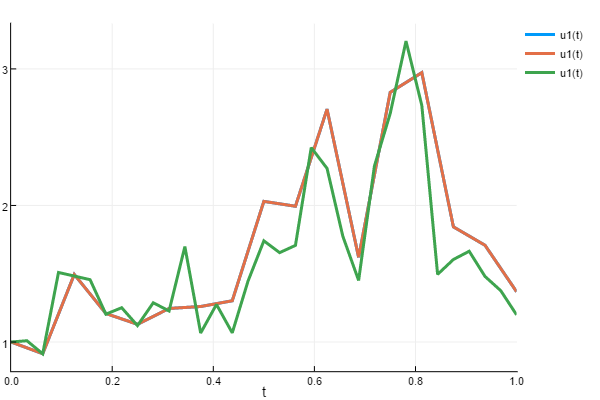
In this plot, sol2 covers up sol1 because they hit essentially the same values. You can see that sol3 is similar to the others, because it's using the same underlying noise process, just sampled much finer.
To double-check, we see that:
plot(sol1.W)
plot!(sol2.W)
plot!(sol3.W)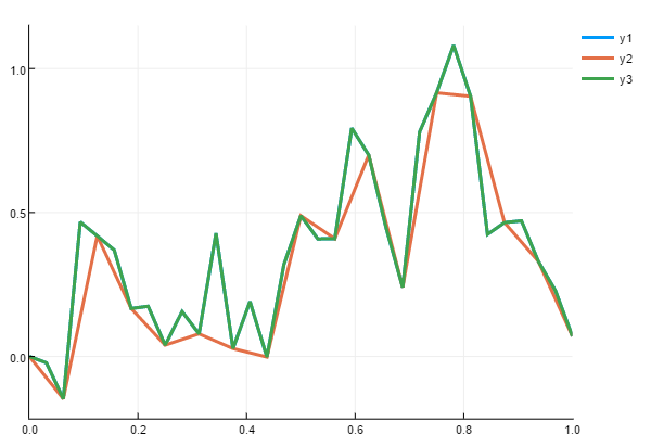
the coupled Wiener processes coincide at every other time point, and the intermediate timepoints were calculated according to a Brownian bridge.
Adaptive NoiseWrapper Example
Here we will show that the same noise can be used with the adaptive methods using the NoiseWrapper. SRI and SRIW1 use slightly different error estimators, and thus have slightly different stepping behavior. We can see how they solve the same 2D SDE differently by using the noise wrapper:
prob = SDEProblem(f1, g1, ones(2), (0.0, 1.0))
sol4 = solve(prob, SRI(), abstol = 1e-8, save_noise = true)

W2 = NoiseWrapper(sol4.W)
prob2 = SDEProblem(f1, g1, ones(2), (0.0, 1.0), noise = W2)
sol5 = solve(prob2, SRIW1(), abstol = 1e-8)

using Plots
plot(sol4)
plot!(sol5)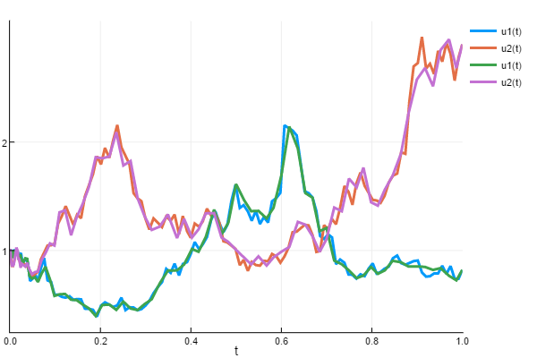
Noise Functions
DiffEqNoiseProcess.NoiseFunction — Type
NoiseFunction{T, N, wType, zType, Tt, T2, T3, inplace} <:
AbstractNoiseProcess{T, N, nothing, inplace}
This allows you to use any arbitrary function W(t) as a NoiseProcess. This will use the function lazily, only caching values required to minimize function calls, but not storing the entire noise array. This requires an initial time point t0 in the domain of W. A second function is needed if the desired SDE algorithm requires multiple processes.
NoiseFunction{iip}(t0, W, Z = nothing;
    noise_prototype = W(nothing, nothing, t0),
    reset = true) where {iip}
Arguments
t0: Initial time.W: Primary function, called asW(u, p, t)orW(out, u, p, t).Z: Optional auxiliary function with the same calling convention.
Keywords
noise_prototype: Initial value and storage prototype for in-place functions.reset: Whether solving a problem resets the current time and values.
Fields
W,Z: Primary and optional auxiliary functions.t0,curt: Initial and current times.curW,curZ: Current function values.dt,dW,dZ: Proposed step and pending increments.reset: Reset behavior.
NoiseFunction evaluates a deterministic function lazily; it does not retain a complete saved path.
Additionally, one can use an in-place function W(out1,out2,t) for more efficient generation of the arrays for multidimensional processes. When the in-place version is used without a dispatch for the out-of-place version, the noise_prototype needs to be set.
NoiseFunction Example
The NoiseFunction is pretty simple: pass a function. As a silly example, we can use exp as a noise process by doing:
f(u, p, t) = exp(t)
W = NoiseFunction(0.0, f)
If it's multidimensional and an in-place function is used, the noise_prototype must be given. For example:
f(out, u, p, t) = (out .= exp(t))
W = NoiseFunction(0.0, f, noise_prototype = rand(4))
This allows you to put arbitrarily weird noise into SDEs and RODEs. Have fun.
DiffEqNoiseProcess.NoiseTransport — Type
NoiseTransport{T, N, wType, zType, Tt, T2, T3, TRV, Trv, RNGType, inplace} <:
AbstractNoiseProcess{T, N, nothing, inplace}
This allows you to define stochastic processes of the form W(t) = f(u, p, t, RV), where f is a function and RV represents a random variable. This will use the function lazily, only caching values required to minimize function calls, but not storing the entire noise array. This requires an initial time point t0 in the domain of W. A second function is needed if the desired SDE algorithm requires multiple processes.
NoiseTransport{iip}(t0,
    W,
    RV,
    rv,
    Z = nothing;
    rng = Random.default_rng(),
    reset = true,
    reseed = true,
    noise_prototype = W(nothing, nothing, t0, rv)) where {iip}
NoiseTransport(t0,
W,
RV;
rng = Random.default_rng(),
reset = true,
reseed = true,
kwargs...)Arguments
t0: Initial time.W: Primary transport function, called asW(u, p, t, rv)orW(out, u, p, t, rv).RV: Random-variable generator, called asRV(rng)orRV(rng, rv).rv: Optional realization or mutable realization prototype.Z: Optional auxiliary transport function.
Keywords
rng: Random number generator used to draw realizations.reset: Whether solving a problem resets the process.reseed: Whether a new realization is drawn when the process is reseeded.noise_prototype: Initial output shape for in-place transport functions.
Fields
W,Z: Primary and optional auxiliary transport functions.RV,rv: Random-variable generator and current realization.curt,curW,curZ: Current time and transported values.rng,reset,reseed: Randomness and reset controls.
Additionally, one can use an in-place function W(out, u, p, t, rv) for more efficient generation of the arrays for multidimensional processes. When the in-place version is used without a dispatch for the out-of-place version, the noise_prototype needs to be set.
NoiseTransport Example
The NoiseTransport requires you to pass an initial time, a transport function, and a random variable. The random variable can be either out-of-place or in-place. It is assumed it is out-of-place when the realization is a subtype of Number, and in-place, when it is a subtype of AbstractArray. Here, a random variable is any function that accepts a random number generator, in the out-of-place case (e.g. rand(rng)), or a random number generator and a realization to be mutated (e.g. rand!(rng, rv)).
An optional realization rv may be given. The realization rv is used in the first time an AbstractRODEProblem is solved. Subsequent runs of the same problem will draw a different realization from the random variable RV, unless reseed is set to false. In the case of a NoiseProblem, however, a new realization will happen at the first run already, and, in this case, rv can be regarded as a realization prototype, which is necessary in the case of a random vector.
As a first example, let us implement the Gaussian noise W(t) = sin(Yt), where Y is a normal random variable.
f(u, p, t, rv) = sin(rv * t)
t0 = 0.0
W = NoiseTransport(t0, f, randn)
If we want to build a scalar random process out of a random vector, then an in-place version of the random vector is required, as follows. We can also use parameters in the transport function, in which case the noise_prototype must be given.
using Random: randn!
f(u, p, t, rv) = sin(p[1] * t + rv[1]) + cos(p[2] * t + rv[2])
t0 = 0.0
rv = randn(2)
p = (π, 2π)
W = NoiseTransport(t0, f, randn!, rv, noise_prototype = f(nothing, p, t0, rv))
If the random process is expected to be multidimensional, it is preferable to use an in-place transport function, and, in this case, the noise_prototype must be given. Here is an example with a scalar random vector with a beta distribution, from Distributions.jl.
f!(out, u, p, t, rv) = (out .= sin.(rv * t))
t0 = 0.0
RV(rng) = rand(rng, Beta(2, 3))
rv = 0.0
W = NoiseTransport(t0, f!, RV, rv, noise_prototype = zeros(4))
We can also have a random vector with a multidimensional process, in which case an in-place version of RV is required. For example.
using Random: randn!

function f!(out, u, p, t, v)
    out[1] = sin(v[1] * t)
    out[2] = sin(t + v[2])
    out[3] = cos(t) * v[1] + sin(t) * v[2]
    nothing
end

t0 = 0.0
RV!(rng, v) = (v[1] = randn(rng); v[2] = rand(rng))
rv = zeros(2)

W = NoiseTransport(t0, f!, RV!, rv, noise_prototype = zeros(3))
A NoiseTransport can be used as driving noise for SDEs and RODEs. Have fun!
Noise from Data
DiffEqNoiseProcess.NoiseGrid — Type
A noise grid builds a noise process from arrays of points. For example, you can generate your desired noise process as an array W with timepoints t, and use the constructor:
NoiseGrid(t, W, Z = nothing; reset = true)to build the associated noise process. This process comes with a linear interpolation of the given points, and thus the grid does not have to match the grid of integration. Thus, this can be used for adaptive solutions as well. However, one must take note that the fidelity of the noise process is linked to how fine the noise grid is determined: if the noise grid is sparse on points compared to the integration, then its distributional properties may be slightly perturbed by the linear interpolation. Thus, it's suggested that the grid size at least approximates the number of time steps in the integration to ensure accuracy.
For a one-dimensional process, W should be an AbstractVector of Numbers. For multidimensional processes, W should be an AbstractVector of the noise_prototype.
Arguments
t: Strictly monotone time points.W: Values at the time points, withlength(W) == length(t).Z: Optional auxiliary values with the same time grid.
Keywords
reset: Whether solving a problem resets the current grid position.
Fields
t,W,Z: Input grid and primary/auxiliary values.curt,curW,curZ: Current interpolated position and values.dt,dW,dZ: Proposed step and pending increments.reset: Reset behavior.
Interpolation is linear. A grid is convenient for replaying sampled data, but it is not distributionally exact between sparse points.
NoiseGrid
In this example, we will show you how to define your own version of Brownian motion using an array of pre-calculated points. In normal usage, you should use WienerProcess instead, since this will have distributionally-exact interpolations while the noise grid uses linear interpolations, but this is a nice example of the workflow.
To define a NoiseGrid you need to have a set of time points and a set of values for the process. Let's define a Brownian motion on (0.0,1.0) with a dt=0.001. To do this,
dt = 0.001
t = 0:dt:1
brownian_values = cumsum([0; [sqrt(dt) * randn() for i in 1:(length(t) - 1)]])
Now we build the NoiseGrid using these values:
W = NoiseGrid(t, brownian_values)We can then pass W as the noise argument of an SDEProblem to use it in an SDE.
Noise Approximation
DiffEqNoiseProcess.NoiseApproximation — Type
In many cases, one would like to define a noise process directly by a stochastic differential equation which does not have an analytical solution. Of course, this will not be distributionally-exact and how well the properties match depends on how well the differential equation is integrated, but in many cases , this can be used as a good approximation when other methods are much more difficult.
A NoiseApproximation is defined by a DEIntegrator. The constructor for a NoiseApproximation is:
NoiseApproximation(source1::DEIntegrator,
    source2::Union{DEIntegrator, Nothing} = nothing;
    reset = true)
The DEIntegrator should have a final time point of integration far enough away, such that it will not halt during the integration. For ease of use, you can use a final time point as Inf. Note that the time points do not have to match the time points of the future integration, since the interpolant of the SDE solution will be used. Thus, the limiting factor is error tolerance, and not hitting specific points.
Arguments
source1: InitializedDEIntegratorproviding the primary noise path.source2: Optional second integrator providing the auxiliary path.
Keywords
reset: Whether solving a problem reinitializes both copied integrators.
Fields
source1,source2: Deep-copied integrators used for interpolation.t,W,Z: Saved source time points and values.curt,curW,curZ: Current time and values.reset: Reset behavior.
NoiseApproximation Example
In this example, we will show how to use the NoiseApproximation to build our own Geometric Brownian Motion from its stochastic differential equation definition. In normal usage, you should use the GeometricBrownianMotionProcess instead since that is more efficient and distributionally-exact.
First, let's define the SDEProblem. Here, we use a timespan (0.0,Inf) so that the noise can be used over an indefinite integral.
const μ = 1.5
const σ = 1.2
f(u, p, t) = μ * u
g(u, p, t) = σ * u
prob = SDEProblem(f, g, 1.0, (0.0, Inf))
Now we build the noise process by building the integrator and sending that integrator to the NoiseApproximation constructor:
integrator = init(prob, SRIW1())
W = NoiseApproximation(integrator)
We can use this noise process like any other noise process. For example, we can now build a geometric Brownian motion whose noise process is colored noise that itself is a geometric Brownian motion:
prob = SDEProblem(f, g, 1.0, (0.0, Inf), noise = W)The possibilities are endless.
Memory-Efficient Alternatives
DiffEqNoiseProcess.VirtualBrownianTree — Type
A VirtualBrownianTree builds the noise process starting from an initial time t0, the first value of the process W0, and (optionally) the first value Z0 for an auxiliary pseudo-process. The constructor is given as
VirtualBrownianTree(t0,
    W0,
    Z0 = nothing,
    dist = WHITE_NOISE_DIST,
    bridge = VBT_BRIDGE;
    kwargs...)
where dist specifies the distribution that is used to generate the end point(s) Wend (Zend) of the noise process for the final time tend. bridge denotes the distribution of the employed Brownian bridge. Per default tend is fixed to t0+1 but can be changed by passing a custom tend as a keyword argument. The following keyword arguments are available:
tendis the end time of the noise process.Wendis the end value of the noise process.Zendis the end value of the pseudo-noise process.atolrepresents the absolute tolerance determining when the recursion is terminated.tree_depthallows one to store a cache of seeds, noise values, and times to speed up the simulation by reducing the recursion steps.search_depthmaximal search depth for the tree ifatolis not reached.rngthe splittable PRNG used for generating the random numbers. Default:Xoshiro()from the Random package.
Fields
dist,bridge: Endpoint distribution and bridge callbacks.t,W,Z: Cached endpoints and auxiliary values.curt,curW,curZ: Current time and values.dt,dW,dZ: Proposed step and pending increments.seeds: Integer seeds used to make recursive bridge queries reproducible.atol,tree_depth,search_depth,rng: Accuracy, cache, search, and random-generation controls.
The recursive cache and scratch buffers are implementation details; use the callable and step interfaces rather than mutating them directly.
VirtualBrownianTree Example
In this example, we define a multidimensional Brownian process based on a VirtualBrownianTree with a minimal tree_depth=0 such that memory consumption is minimized.
W0 = zeros(10)
W = VirtualBrownianTree(0.0, W0; tree_depth = 0)

prob = NoiseProblem(W, (0.0, 1.0))
sol = solve(prob; dt = 1 / 10)
Using a look-up cache by increasing tree_depth can significantly reduce the runtime. Thus, the VirtualBrownianTree allows for trading off speed for memory in a simple manner.
DiffEqNoiseProcess.VirtualBrownianTree! — Function
VirtualBrownianTree!(t0, W0, Z0 = nothing,
    dist = INPLACE_WHITE_NOISE_DIST, bridge = INPLACE_VBT_BRIDGE; kwargs...)
Construct an in-place VirtualBrownianTree noise process.
This is the mutating-distribution variant of VirtualBrownianTree. It uses dist and bridge functions that write noise increments into their output argument, which is useful when W0 is an array-like noise prototype.
DiffEqNoiseProcess.BoxWedgeTail — Type
BoxWedgeTail{T, N, Tt, TA, T2, T3, ZType, F, F2, inplace, RNGType, tolType, spacingType,
    jpdfType, boxType, wedgeType, tailType, distBWTType, distΠType} <:
AbstractNoiseProcess{T, N, Vector{T2}, inplace}
The method for random generation of stochastic area integrals due to Gaines and Lyons. The method is based on Marsaglia's "rectangle-wedge-tail" approach for two dimensions.
3 different groupings for the boxes are implemented.
- box_grouping = :Columns (full, i.e., as large as possible, columns on a square spanned by dr and da)
- box_grouping = :none (no grouping)
- box_grouping = :MinEntropy (default, grouping that achieves a smaller entropy than the column wise grouping and thus allows for slightly faster sampling – but has a slightly larger number of groups)
The sampling is based on the Distributions.jl package, i.e., to sample from one of the many distributions, a uni-/bi-variate distribution from Distributions.jl is constructed, and then rand(..) is used.
Constructor
BoxWedgeTail{iip}(t0, W0, Z0, dist, bridge;
    rtol = 1e-8, nr = 4, na = 4, nz = 10,
    box_grouping = :MinEntropy,
    sqeezing = true,
    save_everystep = true,
    rng = Random.default_rng(),
    reset = true, reseed = true) where {iip}
Arguments
t0: Initial time.W0: Two-dimensional Brownian initial value.Z0: Optional auxiliary process value.dist,bridge: In-place or out-of-place increment callbacks.
Keywords
rtol: Relative tolerance used to build the stochastic-area density.nr,na,nz: Discretization levels for radius, angle, and tail grids.box_grouping::MinEntropy,:Columns, or:none.sqeezing: Whether the wedge sampler uses squeezing bounds.save_everystep,rng,reset,reseed: Standard process controls.
Fields
t,W,Z: Saved times and primary/auxiliary values.A: Saved stochastic-area values.curt,curW,curZ,curA: Current state.rtol,Δr,Δa,Δz: Stochastic-area discretization controls.boxes,wedges,tails: Sampling tables used by the implementation.
The sampling tables are generated data, not extension points. Use the process and step interfaces rather than mutating them directly.
DiffEqNoiseProcess.BoxWedgeTail! — Function
BoxWedgeTail!(t0, W0, Z0 = nothing,
    dist = INPLACE_WHITE_NOISE_DIST, bridge = INPLACE_WHITE_NOISE_BRIDGE; kwargs...)
Construct an in-place BoxWedgeTail noise process.
This is the mutating-distribution variant of BoxWedgeTail for two-dimensional Brownian processes with stochastic area. The supplied dist and bridge functions must write their increments into the provided output arrays.
Preconditioned Crank-Nicolson
DiffEqNoiseProcess.pCN — Function
pCN(noise::AbstractNoiseProcess, ρ; reset=true,reverse=false,indx=nothing)Create a correlated noise proposal from a copy of noise using the preconditioned Crank–Nicolson update. The input process is not mutated.
Arguments
noise: SourceAbstractNoiseProcesswith a saved path.ρ: Correlation parameter, normally in[-1, 1].
Keywords
reset: Whether the returned wrapper resets before solving.reverse: Whether the returned wrapper traverses the source backwards.indx: Initial source index for the wrapper.
Returns
A NoiseWrapper containing the correlated proposal.
Example
W = WienerProcess(0.0, 0.0)
proposal = pCN(W, 0.9)pCN(noise::NoiseGrid, ρ; reset=true, rng = Random.default_rng())Create a correlated proposal from a NoiseGrid. The source grid is not mutated; the returned grid has the same time points and auxiliary process.
Arguments
noise: SourceNoiseGrid.ρ: Correlation parameter, normally in[-1, 1].
Keywords
reset: Reset flag stored on the returned grid.rng: Random number generator used for the innovation.
Returns
A new NoiseGrid containing the correlated proposal.
Example
grid = NoiseGrid(0.0:0.1:1.0, zeros(11))
proposal = pCN(grid, 0.9)
External links
DiffEqNoiseProcess.pCN! — Function
pCN!(noise::AbstractNoiseProcess, ρ; reset=true,reverse=false,indx=nothing)Create a correlated noise proposal in-place using the preconditioned Crank–Nicolson update. The source path is replaced by ρ * source + sqrt(1 - ρ^2) * innovation.
Arguments
noise: SourceAbstractNoiseProcesswhose saved path is updated.ρ: Correlation parameter, normally in[-1, 1].
Keywords
reset: Whether the returned wrapper resets before solving.reverse: Whether the returned wrapper traverses the source backwards.indx: Initial source index for the wrapper; defaults to the start (or end whenreverse = true).
Returns
A NoiseWrapper around the updated source. The source itself is mutated.
Example
W = WienerProcess(0.0, 0.0)
proposal = pCN!(W, 0.9)
External links