Discrete Empirical Interpolation Method (DEIM)

This section illustrates how ModelOrderReduction.jl can be used to build a reduced order model via Petrov-Galerkin projection using the Proper Orthogonal Decomposition (POD) and the Discrete Empirical Interpolation Method (DEIM). As an illustrative example, we consider a nonlinear 1-D PDE from the realm of neuroscience.

The FitzHugh-Nagumo system used in neuron modeling is a simplified version of the Hodgkin-Huxley model, which describes in a detailed manner, the activation and deactivation dynamics of a spiking neuron. The system is given as follows. For $x\in [0,L], t\geq 0$,

\[\begin{aligned} \varepsilon v_t(x,t)&=\varepsilon^2 v_{xx}(x,t)+f(v(x,t))-w(x,t)+c,\\ w_t(x,t)&=bv(x,t)-\gamma w(x,t)+c, \end{aligned}\]

with the nonlinear function $f(v)=v(v-0.1)(1-v)$. The initial and boundary conditions are

\[\begin{aligned} v(x,0)=0,\quad w(x,0)=0,\quad x\in [0,L],\\ v_x(0,t)=-i_0(t),\quad v_x(L,t)=0,\quad t\geq 0, \end{aligned}\]

where the parameters are $L=1$, $\varepsilon=0.015$, $b=0.5$, $\gamma =2$, $c=0.05$. The stimulus is $i_0(t)=50000t^3\exp(-15t)$. The variables $v$ and $w$ are voltage and recovery of voltage, respectively.

To generate a POD-DEIM reduced-order model, we need to work through the following steps:

Collect data on full-order model trajectories and the nonlinear terms describing its evolution equation along the way.
Based on the collected data, use POD to identify a low dimensional linear subspace of the system's state space that allows for embedding the full-order model's trajectories with minimal error.
Project the model onto the identified subspace using DEIM to approximate nonlinear terms.

For step 1, we first construct a ModelingToolkit.PDESystem describing the original FitzHugh-Nagumo model.

using ModelingToolkit
using LaTeXStrings
@independent_variables x t
@variables v(..) w(..)
Dx = Differential(x)
Dxx = Dx^2
Dt = Differential(t)
const L = 1.0
const ε = 0.015
const b = 0.5
const γ = 2.0
const c = 0.05
f(v) = v * (v - 0.1) * (1.0 - v)
i₀(t) = 50000.0t^3 * exp(-15.0t)
eqs = [ε * Dt(v(x, t)) ~ ε^2 * Dxx(v(x, t)) + f(v(x, t)) - w(x, t) + c,
    Dt(w(x, t)) ~ b * v(x, t) - γ * w(x, t) + c]
bcs = [v(x, 0.0) ~ 0.0,
    w(x, 0) ~ 0.0,
    Dx(v(0, t)) ~ -i₀(t),
    Dx(v(L, t)) ~ 0.0]
domains = [x ∈ (0.0, L),
    t ∈ (0.0, 14.0)]
ivs = [x, t]
dvs = [v(x, t), w(x, t)]
pde_sys = PDESystem(eqs, bcs, domains, ivs, dvs; name = Symbol("FitzHugh-Nagumo"))

Next, we apply finite difference discretization using MethodOfLines.jl. MethodOfLines v1 constructs an array-form DAEProblem directly. Setting fallback = false keeps this path explicit and avoids compiling a scalarized full-order ODE system.

using MethodOfLines
using SciMLBase: discretize
N = 15 # equidistant discretization intervals
dx = (L - 0.0) / N
dxs = [x => dx]
order = 2
discretization = MOLFiniteDifference(dxs, t; approx_order = order)
full_prob = discretize(pde_sys, discretization; fallback = false)

The snapshot trajectories are obtained by solving the full-order DAE with its default solver.

using DifferentialEquations
sol = solve(full_prob)
sol_x = sol[x]
nₓ = length(sol_x) # number of discretization points in x
nₜ = length(sol[t]) # number of discretization points in time

Let's see the fast decay of the singular values of the snapshot solutions for $v$, $w$, and the nonlinear snapshots $f(v)$.

using LinearAlgebra
snapshot_v = sol[v(x, t)]
snapshot_w = sol[w(x, t)]
snapshot_fv = f.(snapshot_v)
svdval_v = svdvals(snapshot_v)
svdval_w = svdvals(snapshot_w)
svdval_fv = svdvals(snapshot_fv)
using Plots, LaTeXStrings
svd_plt = plot(yscale = :log10, xticks = eachindex(svdval_v), titlefont = 11,
    legendfont = 10, title = "Singular values of the snapshots")
plot!(svd_plt, svdval_v, markershape = :circle, label = L"Singular Val of $v$")
plot!(svd_plt, svdval_w, markershape = :circle, label = L"Singular Val of $w$")
plot!(svd_plt, svdval_fv, markershape = :circle, label = L"Singular Val of $f(v)$")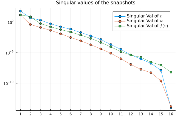

The following figure shows the phase-space diagram of $v$ and $w$ at different spatial points $x$ from the full-order system.

full_plt = plot(xlabel = L"v(x,t)", ylabel = L"x", zlabel = L"w(x,t)", xlims = (-0.5, 2.0),
    ylims = (0.0, L), zlims = (0.0, 0.25), legend = false, xflip = true,
    camera = (50, 30), titlefont = 10,
    title = "Phase−Space diagram of full $(nameof(pde_sys)) system")
@views for i in 1:nₓ
    plot!(full_plt, snapshot_v[i, :], _ -> sol_x[i], snapshot_w[i, :])
end
plot!(full_plt)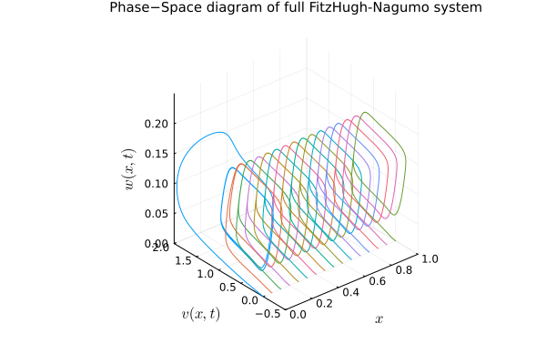

Then, we use POD to construct a linear subspace of dimension, say, 5 for the system's state space and project the model onto the subspace. DEIM is employed to approximate nonlinear terms. This can be done by simply calling deim.

using ModelOrderReduction
pod_dim = deim_dim = 5
deim_sys = deim(full_prob, sol, pod_dim; deim_dim = deim_dim)
deim_prob = DAEProblem(deim_sys, nothing; build_initializeprob = false)
deim_sol = solve(deim_prob)
nₜ_deim = length(deim_sol[t])
sol_deim_x = deim_sol[x]
sol_deim_v = deim_sol[v(x, t)]
sol_deim_w = deim_sol[w(x, t)]

The ROM retains one array differential equation and one reconstruction array per PDE field. For fixed POD/DEIM dimensions, field count, forcing expression count, and local nonlinear stencil size, the generated symbolic graph is independent of the spatial grid. A DAEProblem with build_initializeprob = false generates array code directly from that graph. Alternatively, call mtkcompile on the reduced system and construct an ODEProblem; this scalarizes the reduced differential equation, whose size is fixed by the POD dimension, while the array reconstruction equations are kept.

This compilation bound does not cover offline structural elimination, POD/DEIM training, problem construction, or full-field evaluation. The reconstruction matrix requires O(nk) storage. Differential states use the POD lift; eliminated algebraic states use a least-squares fit to the training snapshots, so reconstructed boundary constraints are approximate. The DAE must reduce to an explicit first-order ODE after algebraic elimination. General descriptor-DAE projection is not implemented by this method.

For a symbolic array field outside the PDE solution interface, construct its array reconstruction function with SymbolicIndexingInterface.observed(deim_sys, field) and evaluate it with (reduced_state, parameters, time). Convenience sol[field] indexing currently has an upstream array-observable issue. The PDE field indexing used in this tutorial uses the explicit reconstruction path.

And plot the result from the POD-DEIM reduced system.

deim_plt = plot(xlabel = L"v(x,t)", ylabel = L"x", zlabel = L"w(x,t)", xlims = (-0.5, 2.0),
    ylims = (0.0, L), zlims = (0.0, 0.25), legend = false, xflip = true,
    camera = (50, 30), titlefont = 10,
    title = "Phase−Space diagram of reduced $(nameof(pde_sys)) system")
@views for i in 1:nₓ
    plot!(deim_plt, sol_deim_v[i, :], _ -> sol_deim_x[i], sol_deim_w[i, :])
end
plot!(deim_plt)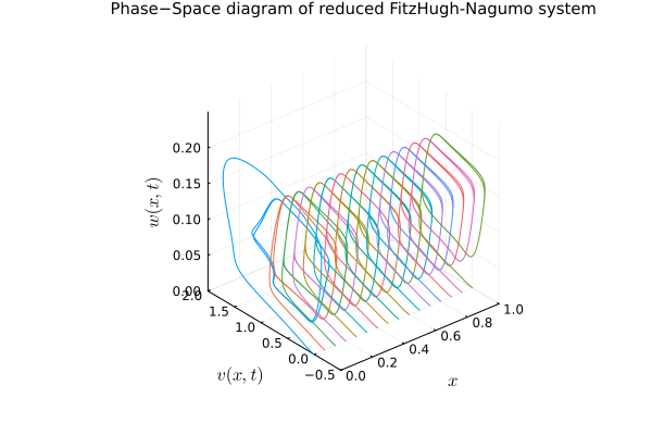

Finally, we put the two solutions into one figure.

# create data for plotting unconnected lines
function unconnected(m::AbstractMatrix)
    row, col = size(m)
    data = similar(m, row, col + 1)
    data[:, begin:(end - 1)] .= m
    data[:, end] .= NaN # path separator
    vec(data')
end
function unconnected(v::AbstractVector, nₜ::Integer)
    data = similar(v, nₜ + 1, length(v))
    for (i, vᵢ) in enumerate(v)
        data[begin:(end - 1), i] .= vᵢ
    end
    data[end, :] .= NaN
    vec(data)
end
plt_2 = plot(xlabel = L"v(x,t)", ylabel = L"x", zlabel = L"w(x,t)", xlims = (-0.5, 2.0),
    ylims = (0.0, L), zlims = (0.0, 0.25), xflip = true, camera = (50, 30),
    titlefont = 10, title = "Comparison of full and reduced systems")
plot!(plt_2, unconnected(snapshot_v), unconnected(sol_x, nₜ), unconnected(snapshot_w),
    label = "Full$(length(full_prob.u0))")
plot!(plt_2, unconnected(sol_deim_v), unconnected(sol_deim_x, nₜ_deim),
    unconnected(sol_deim_w), label = "POD$(pod_dim)/DEIM$(deim_dim)")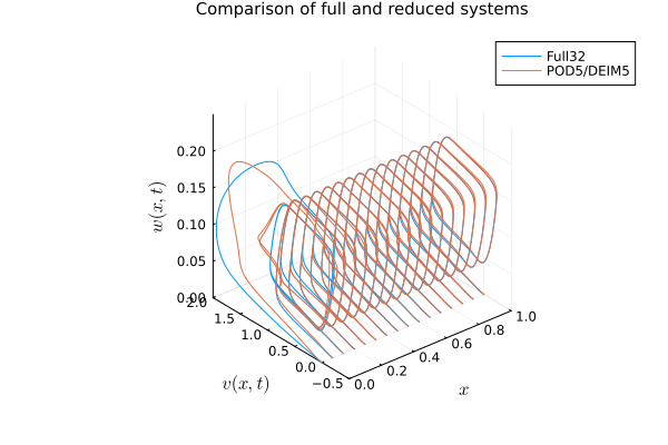

As we can see, the reduced-order system captures the limit cycle of the original full-order system very well.