Solving Dynamic Optimization Problems
Systems in ModelingToolkit.jl can be directly converted to dynamic optimization or optimal control problems. In such systems, one has one or more input variables that are externally controlled to control the dynamics of the system. A dynamic optimization solves for the optimal time trajectory of the input variables in order to maximize or minimize a desired objective function. For example, a car driver might like to know how to step on the accelerator if the goal is to finish a race while using the least gas.
To begin, let us take a rocket launch example. The input variable here is the thrust exerted by the engine. The rocket state is described by its current height, mass, and velocity. The mass decreases as the rocket loses fuel while thrusting.
using ModelingToolkit, OrdinaryDiffEq
t = ModelingToolkit.t_nounits
D = ModelingToolkit.D_nounits

@parameters h_c m₀ h₀ g₀ D_c c Tₘ m_c
@variables begin
    h(..)
    v(..)
    m(..), [bounds = (m_c, 1)]
    T(..), [input = true, bounds = (0, Tₘ)]
end

drag(h, v) = D_c * v^2 * exp(-h_c * (h - h₀) / h₀)
gravity(h) = g₀ * (h₀ / h)

eqs = [D(h(t)) ~ v(t),
    D(v(t)) ~ (T(t) - drag(h(t), v(t))) / m(t) - gravity(h(t)),
    D(m(t)) ~ -T(t) / c]

(ts, te) = (0.0, 0.2)
costs = [-h(te)]
cons = [T(te) ~ 0, m(te) ~ m_c]

@named rocket = System(eqs, t; costs, constraints = cons)
rocket = mtkcompile(rocket, inputs = [T(t)])

u0map = [h(t) => h₀, m(t) => m₀, v(t) => 0]
pmap = [
    g₀ => 1, m₀ => 1.0, h_c => 500, c => 0.5 * √(g₀ * h₀), D_c => 0.5 * 620 * m₀ / g₀,
    Tₘ => 3.5 * g₀ * m₀, T(t) => 0.0, h₀ => 1, m_c => 0.6]
9-element Vector{Pair{Num, Num}}:
g₀ => 1
m₀ => 1.0
h_c => 500
c => 0.5sqrt(g₀*h₀)
D_c => (310.0m₀) / g₀
Tₘ => 3.5g₀*m₀
T(t) => 0.0
h₀ => 1
m_c => 0.6What we would like to optimize here is the final height of the rocket. We do this by providing a vector of expressions corresponding to the costs. By default, the sense of the optimization is to minimize the provided cost. So to maximize the rocket height at the final time, we write -h(te) as the cost.
Now we can construct a problem and solve it. Let us use JuMP as our backend here. Note that the package trigger is actually InfiniteOpt, and not JuMP - this package includes JuMP but is designed for optimization on function spaces. Additionally we need to load the solver package - we will use Ipopt here (a good choice in general).
The collocation solver uses a default ODE tableau. A custom tableau can still be supplied when needed.
import InfiniteOpt, Ipopt
jprob = JuMPDynamicOptProblem(rocket, [u0map; pmap], (ts, te); dt = 0.001)
jsol = solve(jprob, JuMPCollocation(Ipopt.Optimizer));
The solution has three fields: jsol.sol is the ODE solution for the states, jsol.input_sol is the ODE solution for the inputs, and jsol.model is the wrapped model that we can use to query things like objective and constraint residuals.
Let's plot the final solution and the controller here:
using CairoMakie
fig = Figure(resolution = (800, 400))
ax1 = Axis(fig[1, 1], title = "Rocket trajectory", xlabel = "Time")
ax2 = Axis(fig[1, 2], title = "Control trajectory", xlabel = "Time")

for u in unknowns(rocket)
    lines!(ax1, jsol.sol.t, jsol.sol[u], label = string(u))
end
lines!(ax2, jsol.input_sol, label = "Thrust")
axislegend(ax1)
axislegend(ax2)
fig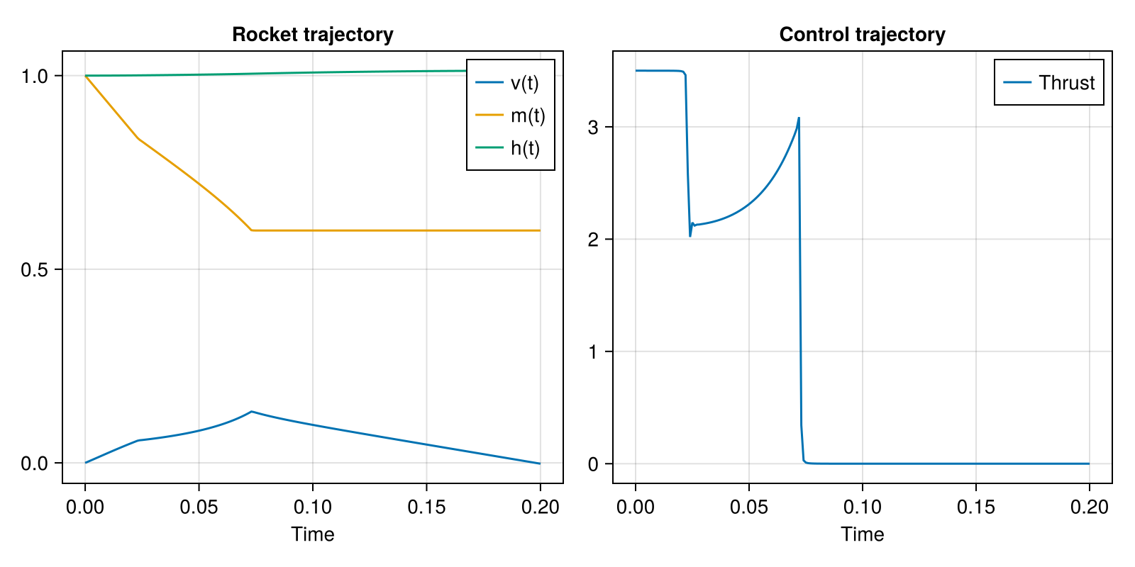
Providing an initial trajectory
By default every state variable is seeded with its constant value from u0map at each collocation point. When that starting point is a poor one, the solver can be given a guess of the whole trajectory instead. The initial_trajectory keyword takes a map from states to symbolic expressions in the independent variable:
jprob_guess = JuMPDynamicOptProblem(rocket, [u0map; pmap], (ts, te); dt = 0.001,
    initial_trajectory = Dict(h(t) => 1 + t, v(t) => 1.0))
jsol_guess = solve(jprob_guess, JuMPCollocation(Ipopt.Optimizer));
Each expression is compiled to a function and evaluated at the collocation points to produce the start values handed to the optimizer. Only the states listed are affected — the rest keep their constant seed. This changes where the solve starts from, not the optimum it converges to.
Expressions may reference parameters, which are resolved from the operating point, so the guess can be written in terms of the same quantities as the model:
jprob_guess2 = JuMPDynamicOptProblem(rocket, [u0map; pmap], (ts, te); dt = 0.001,
    initial_trajectory = Dict(h(t) => h₀ + t, v(t) => t))
jsol_guess2 = solve(jprob_guess2, JuMPCollocation(Ipopt.Optimizer));
Only parameters of the compiled system can be referenced this way; anything else — another state, or a quantity mtkcompile has eliminated that does not reduce to time and parameters — raises an ArgumentError naming the unresolved quantity.
initial_trajectory is supported by the JuMP, InfiniteOpt, and CasADi backends. Passing a non-empty map to Pyomo raises an ArgumentError.
For free final time problems (see below) the collocation grid is normalized to [0, 1], so the trajectory expressions are evaluated at normalized time rather than physical time.
Scaling the dynamics constraints
When the states of a system span very different magnitudes, the residuals of the dynamics constraints do too, which can make the optimizer favor the large states and converge poorly. The nominal_values keyword takes a map from states to their typical magnitudes, and each dynamics constraint is divided by the corresponding value so that all residuals are comparable in size:
iprob_scaled = InfiniteOptDynamicOptProblem(rocket, [u0map; pmap], (ts, te); dt = 0.001,
    nominal_values = Dict(h(t) => 1.25, m(t) => 0.6))
isol_scaled = solve(iprob_scaled, InfiniteOptCollocation(Ipopt.Optimizer));
States not listed default to their nominal metadata if set, and to 1.0 otherwise, in which case the constraint is unchanged. Scaling a residual does not move the optimum, only how the solver converges towards it.
nominal_values affects the InfiniteOpt and Pyomo backends, which emit the dynamics directly as derivative constraints. The JuMP and CasADi backends discretize through an ODE solver tableau instead and currently ignore it.
Bounds on observed variables
Bounds declared on an observed variable are enforced too, not just bounds on states and inputs. Here the observed power is capped, which limits how hard the input may drive the state:
@variables begin
    z(..)
    power(..), [bounds = (0.0, 1.0)]
    w(..), [input = true, bounds = (-1.0, 1.0)]
end

@named limited = System(
    [D(z(t)) ~ w(t), power(t) ~ 2z(t)], t; costs = [-z(1.0)])
limited = mtkcompile(limited; inputs = [w(t)])

lprob = JuMPDynamicOptProblem(
    limited, [[z(t) => 0.0]; [w(t) => 0.0]], (0.0, 1.0); dt = 0.01)
lsol = solve(lprob, JuMPCollocation(Ipopt.Optimizer));
lsol.sol[z(t)][end] # 0.5, not 1.0: power = 2z ≤ 1 binds0.5000000043694979There are two ways to impose such a bound, selected with observed_bounds_method:
:liftintroduces an auxiliary decision variable bounded by[lo, hi]and ties it to the observed expression with an equality constraint. Interior-point solvers such as Ipopt handle variable bounds considerably better than the equivalent nonlinear inequalities, so this is usually faster. Not every backend can do it.:constraintemits the bound directly as a nonlinear inequality. Every backend supports this.:auto, the default, uses:liftwhere the backend supports it and:constrainteverywhere else.
Currently only the JuMP and InfiniteOpt backends can lift; CasADi and Pyomo use :constraint. Asking a backend for :lift when it cannot raises an ArgumentError rather than silently doing something else.
:constraint is worth choosing explicitly when the solver is not interior-point (active set and SQP methods handle inequalities natively), when there are many bounded observed variables and the extra equality constraints make finding an initial feasible point harder, or when comparing against a reference formulation.
Free final time problems
There are additionally a class of dynamic optimization problems where we would like to know how to control our system to achieve something in the least time. Such problems are called free final time problems, since the final time is unknown. To model these problems in ModelingToolkit, we declare the final time as a parameter.
Below we have a model system called the double integrator. We control the acceleration of a block in order to reach a desired destination in the least time.
@variables begin
    x(..)
    v(..)
    u(..), [bounds = (-1.0, 1.0), input = true]
end

@parameters tf

constr = [v(tf) ~ 0, x(tf) ~ 0]
cost = [tf] # Minimize time

@named block = System(
    [D(x(t)) ~ v(t), D(v(t)) ~ u(t)], t; costs = cost, constraints = constr)

block = mtkcompile(block; inputs = [u(t)])

u0map = [x(t) => 1.0, v(t) => 0.0]
tspan = (0.0, tf)
parammap = [u(t) => 0.0, tf => 1.0]
2-element Vector{Pair{Num, Float64}}:
u(t) => 0.0
tf => 1.0The tf mapping in the parameter map is treated as an initial guess.
Please note that, at the moment, free final time problems cannot support constraints defined at definite time values, like x(3) ~ 2.
The Pyomo collocation methods (LagrangeRadau, LagrangeLegendre) currently are bugged for free final time problems. Strongly suggest using BackwardEuler() for such problems when using Pyomo as the backend.
When declaring the problem in this case we need to provide the number of steps, since dt can't be known in advanced. Let's solve plot our final solution and the controller for the block, using InfiniteOpt as the backend:
iprob = InfiniteOptDynamicOptProblem(block, [u0map; parammap], tspan; steps = 100)
isol = solve(iprob, InfiniteOptCollocation(Ipopt.Optimizer));
Let's plot the final solution and the controller here:
fig = Figure(resolution = (800, 400))
ax1 = Axis(fig[1, 1], title = "Block trajectory", xlabel = "Time")
ax2 = Axis(fig[1, 2], title = "Control trajectory", xlabel = "Time")

for u in unknowns(block)
    lines!(ax1, isol.sol.t, isol.sol[u], label = string(u))
end
lines!(ax2, isol.input_sol, label = "Acceleration")
axislegend(ax1)
axislegend(ax2)
fig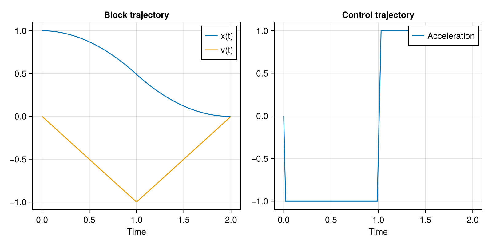
Parameter estimation
The dynamic optimization framework can also be used for parameter estimation. In this approach, we treat unknown parameters as tunable variables and minimize the difference between model predictions and observed data.
Let's demonstrate this with the Lotka-Volterra equations. First, we'll generate some synthetic data by solving the system with known parameter values:
@parameters α = 1.5 β = 1.0 [tunable=false] γ = 3.0 δ = 1.0
@variables x_pe(t) y_pe(t)

eqs_pe = [D(x_pe) ~ α * x_pe - β * x_pe * y_pe,
    D(y_pe) ~ -γ * y_pe + δ * x_pe * y_pe]

@mtkcompile sys0_pe = System(eqs_pe, t)
tspan_pe = (0.0, 1.0)
u0map_pe = [x_pe => 4.0, y_pe => 2.0]

# True parameter values (these are what we'll try to recover)
parammap_pe = [α => 2.5, δ => 1.8]

oprob_pe = ODEProblem(sys0_pe, [u0map_pe; parammap_pe], tspan_pe)
osol_pe = solve(oprob_pe, Tsit5())

# Generate synthetic data at 51 time points
ts_pe = range(tspan_pe..., length=51)
data_pe = osol_pe(ts_pe, idxs=x_pe).u
51-element Vector{Float64}:
4.0
4.033188529297993
4.051589539498085
4.0535385305548255
4.037525368230605
4.0022875247869685
3.946984767817523
3.8712447408627892
3.7752731693385577
3.659977816802768
⋮
0.521087203442534
0.509932674972921
0.5004714566378289
0.4925705181014686
0.48612035236018386
0.4810222214807002
0.4771832830626636
0.4745274362929259
0.47298920296524505Now we'll set up the parameter estimation problem. We use EvalAt to evaluate the state at specific time points and construct a least-squares cost function:
costs_pe = [abs2(EvalAt(ti)(x_pe) - data_pe[i]) for (i, ti) in enumerate(ts_pe)]

@mtkcompile sys_pe = System(eqs_pe, t; costs = costs_pe)
\[ \begin{align} \frac{\mathrm{d} ~ \mathtt{y\_pe}\left( t \right)}{\mathrm{d}t} &= - \mathtt{y\_pe}\left( t \right) ~ \gamma + \mathtt{x\_pe}\left( t \right) ~ \mathtt{y\_pe}\left( t \right) ~ \delta \\ \frac{\mathrm{d} ~ \mathtt{x\_pe}\left( t \right)}{\mathrm{d}t} &= \mathtt{x\_pe}\left( t \right) ~ \alpha - \mathtt{x\_pe}\left( t \right) ~ \mathtt{y\_pe}\left( t \right) ~ \beta \end{align} \]
By default the cost values are sumed up, if a different behaviour is desired, the consolidate keyword can be set in the System definition.
Next, we select which parameters to tune using subset_tunables. Here we'll estimate α and δ while keeping β and γ fixed:
sys_pe′ = subset_tunables(sys_pe, [α, δ])\[ \begin{align} \frac{\mathrm{d} ~ \mathtt{y\_pe}\left( t \right)}{\mathrm{d}t} &= - \mathtt{y\_pe}\left( t \right) ~ \gamma + \mathtt{x\_pe}\left( t \right) ~ \mathtt{y\_pe}\left( t \right) ~ \delta \\ \frac{\mathrm{d} ~ \mathtt{x\_pe}\left( t \right)}{\mathrm{d}t} &= \mathtt{x\_pe}\left( t \right) ~ \alpha - \mathtt{x\_pe}\left( t \right) ~ \mathtt{y\_pe}\left( t \right) ~ \beta \end{align} \]
Now we can solve the parameter estimation problem. Note the tune_parameters=true flag:
iprob_pe = InfiniteOptDynamicOptProblem(sys_pe′, u0map_pe, tspan_pe; dt=1/50, tune_parameters=true)
isol_pe = solve(iprob_pe, InfiniteOptCollocation(Ipopt.Optimizer, InfiniteOpt.OrthogonalCollocation(3)))

println("Estimated α = ", isol_pe.sol.ps[α], " (true value: 2.5)")
println("Estimated δ = ", isol_pe.sol.ps[δ], " (true value: 1.8)")
┌ Warning: No unbound inputs were found in system.
└ @ ModelingToolkitBase ~/work/ModelingToolkit.jl/ModelingToolkit.jl/lib/ModelingToolkitBase/src/inputoutput.jl:266
Estimated α = 2.500470075480321 (true value: 2.5)
Estimated δ = 1.7996676351728234 (true value: 1.8)Let's visualize the fit:
fig = Figure(resolution = (800, 400))
ax = Axis(fig[1, 1], title = "Parameter Estimation Results", xlabel = "Time", ylabel = "Prey Population")
scatter!(ax, ts_pe, data_pe, label = "Data", markersize = 8)
lines!(ax, isol_pe.sol.t, isol_pe.sol[x_pe], label = "Fitted Model", linewidth = 2)
axislegend(ax)
fig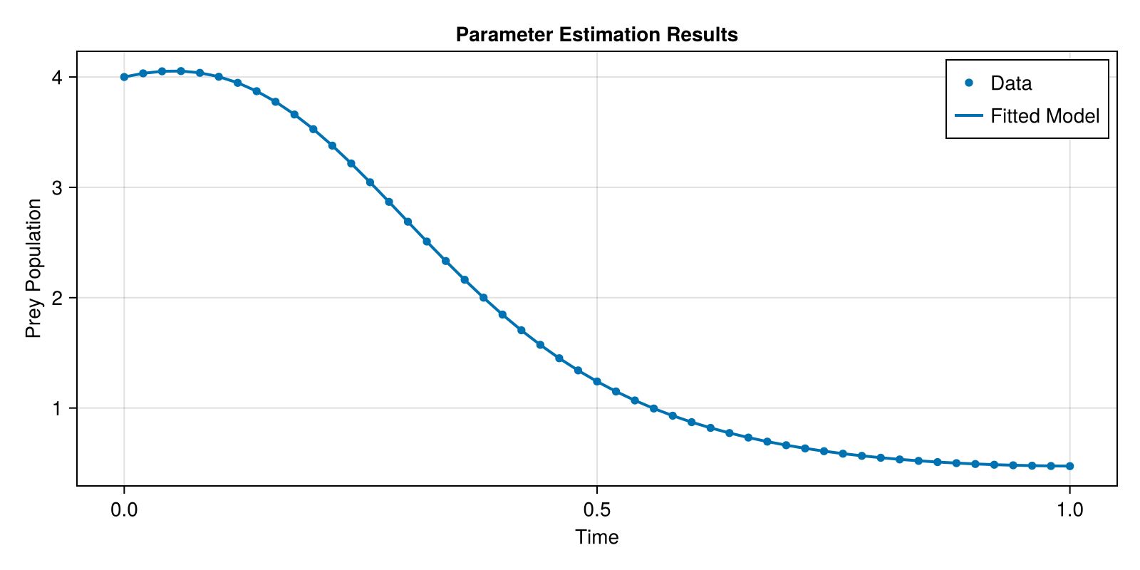
When using EvalAt for parameter estimation, different backends handle the case when evaluation times don't align with collocation points differently:
- JuMP: Will throw an error asking you to adjust
dtif evaluation times don't match collocation points exactly. - CasADi: Uses linear interpolation between collocation points for cost evaluations at intermediate times.
- InfiniteOpt: Automatically adds support points for the evaluation times, handling mismatched grids gracefully.
For example, InfiniteOpt can use a different dt than what the data spacing requires:
# With InfiniteOpt, dt doesn't need to match the data points:
iprob_pe2 = InfiniteOptDynamicOptProblem(sys_pe′, u0map_pe, tspan_pe,
                                         dt = 1/120, tune_parameters=true)
isol_pe2 = solve(iprob_pe2, InfiniteOptCollocation(Ipopt.Optimizer,
                            InfiniteOpt.OrthogonalCollocation(3)))

println("With dt=1/120: Estimated α = ", isol_pe2.sol.ps[α], " (true value: 2.5)")
println("With dt=1/120: Estimated δ = ", isol_pe2.sol.ps[δ], " (true value: 1.8)")
┌ Warning: No unbound inputs were found in system.
└ @ ModelingToolkitBase ~/work/ModelingToolkit.jl/ModelingToolkit.jl/lib/ModelingToolkitBase/src/inputoutput.jl:266
With dt=1/120: Estimated α = 2.5001294315721316 (true value: 2.5)
With dt=1/120: Estimated δ = 1.7999964982431194 (true value: 1.8)This flexibility makes InfiniteOpt particularly convenient for parameter estimation when your data points don't naturally align with a uniform collocation grid.