Linear Analysis

Linear analysis refers to the process of linearizing a nonlinear model and analysing the resulting linear dynamical system. To facilitate linear analysis, ModelingToolkitStandardLibrary provides the concept of an AnalysisPoint, which can be inserted in-between two causal blocks (such as those from the Blocks sub module). Once a model containing analysis points is built, several operations are available:

• get_sensitivity gets the sensitivity function (wiki), $S(s)$, as defined in the field of control theory.
• get_comp_sensitivity gets the complementary sensitivity function $T(s) : S(s)+T(s)=1$.
• get_looptransfer gets the (open) loop-transfer function where the loop starts and ends in the analysis point. For a typical simple feedback connection with a plant $P$ and a controller $C$, the loop-transfer function at the plant output is $P(s)C(s)$.
• linearize can be called with two analysis points denoting the input and output of the linearized system.
• open_loop returns a new nonlinear system where the loop has been broken at the analysis point.

An analysis point can be created explicitly using the AnalysisPoint constructor, or automatically when connecting two causal components using connect:

connect(comp1.output, :analysis_point_name, comp2.input)

The directionality of an analysis point can be thought of as an arrow in a block diagram, where the name of the analysis point applies to the arrow itself.

┌─────┐         ┌─────┐
│     │  name   │     │
│  out├────────►│in   │
│     │         │     │
└─────┘         └─────┘

This is signified by the name being the middle argument to connect.

Of the above mentioned functions, all except for open_loop return the output of ModelingToolkit.linearize, which is

matrices, simplified_sys = linearize(...)
# matrices = (; A, B, C, D)

i.e., matrices is a named tuple containing the matrices of a linear state-space system on the form

\[\begin{aligned} \dot x &= Ax + Bu\\ y &= Cx + Du \end{aligned}\]

Example

The following example builds a simple closed-loop system with a plant $P$ and a controller $C$. Two analysis points are inserted, one before and one after $P$. We then derive a number of sensitivity functions and show the corresponding code using the package ControlSystemBase.jl

using ModelingToolkitStandardLibrary.Blocks, ModelingToolkit
@named P = FirstOrder(k = 1, T = 1) # A first-order system with pole in -1
@named C = Gain(-1)             # A P controller
t = ModelingToolkit.get_iv(P)
eqs = [connect(P.output, :plant_output, C.input)  # Connect with an automatically created analysis point called :plant_output
       connect(C.output, :plant_input, P.input)]
sys = System(eqs, t, systems = [P, C], name = :feedback_system)

matrices_S = get_sensitivity(sys, :plant_input)[1] # Compute the matrices of a state-space representation of the (input)sensitivity function.
matrices_T = get_comp_sensitivity(sys, :plant_input)[1]

(A = [-2.0;;], B = [-1.0;;], C = [-1.0;;], D = [0.0;;])

Continued linear analysis and design can be performed using ControlSystemsBase.jl. We create ControlSystemsBase.StateSpace objects using

using ControlSystemsBase, Plots
S = ss(matrices_S...)
T = ss(matrices_T...)
bodeplot([S, T], lab = ["S" "" "T" ""], plot_title = "Bode plot of sensitivity functions",
    margin = 5Plots.mm)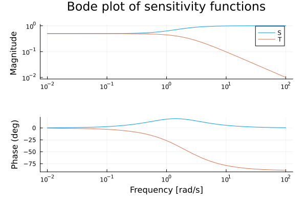

The sensitivity functions obtained this way should be equivalent to the ones obtained with the code below

using ControlSystemsBase
P = tf(1.0, [1, 1]) |> ss
C = 1                      # Negative feedback assumed in ControlSystems
S = sensitivity(P, C)      # or feedback(1, P*C)
T = comp_sensitivity(P, C) # or feedback(P*C)

ControlSystemsBase.StateSpace{ControlSystemsBase.Continuous, Float64}
A = 
 -2.0
B = 
 1.0
C = 
 1.0
D = 
 0.0

Continuous-time state-space model

We may also derive the loop-transfer function $L(s) = P(s)C(s)$ using

matrices_L = get_looptransfer(sys, :plant_output)[1]
L = ss(matrices_L...)

ControlSystemsBase.StateSpace{ControlSystemsBase.Continuous, Float64}
A = 
 -1.0
B = 
 -1.0
C = 
 1.0
D = 
 0.0

Continuous-time state-space model

which is equivalent to the following with ControlSystems

L = P * (-C) # Add the minus sign to build the negative feedback into the controller

ControlSystemsBase.StateSpace{ControlSystemsBase.Continuous, Float64}
A = 
 -1.0
B = 
 -1.0
C = 
 1.0
D = 
 -0.0

Continuous-time state-space model

To obtain the transfer function between two analysis points, we call linearize

matrices_PS = linearize(sys, :plant_input, :plant_output)[1]

(A = [-2.0;;], B = [1.0;;], C = [1.0;;], D = [0.0;;])

this particular transfer function should be equivalent to the linear system P(s)S(s), i.e., equivalent to

feedback(P, C)

ControlSystemsBase.StateSpace{ControlSystemsBase.Continuous, Float64}
A = 
 -2.0
B = 
 1.0
C = 
 1.0
D = 
 0.0

Continuous-time state-space model

Obtaining transfer functions

A statespace system from ControlSystemsBase can be converted to a transfer function using the function tf:

tf(S)

ControlSystemsBase.TransferFunction{ControlSystemsBase.Continuous, ControlSystemsBase.SisoRational{Float64}}
1.0s + 1.0
----------
1.0s + 2.0

Continuous-time transfer function model

Gain and phase margins

Further linear analysis can be performed using the analysis methods from ControlSystemsBase. For example, calculating the gain and phase margins of a system can be done using

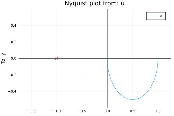
margin(P)

(wgm = [NaN;;], gm = [Inf;;], wpm = [-0.0;;], pm = [180.0;;])

(they are infinite for this system). A Nyquist plot can be produced using

nyquistplot(P)

Index