NBodySimulator.jl

Simulating systems of N interacting bodies.

This project is under development at the moment. The implementation of potential calculations is fairly experimental and has not been extensively verified yet. You can test simulations of different systems now, but be aware of possible changes in the future.

Installation

To install NBodySimulator.jl, use the Julia package manager:

using Pkg
Pkg.add("NBodySimulator")

Basic Components

There are three basic components required for any simulation of systems of N-bodies: bodies, system, and simulation.

Bodies or Particles are the objects that will interact with each other and for which the equations of Newton's 2nd law are solved during the simulation process. Three parameters of a body are necessary, namely: initial location, initial velocity, and mass. MassBody structure represents such particles:

using StaticArrays
r = SVector(0.0, 0.0, 0.0)
v = SVector(0.1, 0.2, 0.5)
mass = 1.25
body = MassBody(r, v, mass)

For simulation speed, it is advised to use static arrays.

A System covers the bodies and the necessary parameters for the correct simulation of interaction between particles. For example, to create an entity for a system of gravitationally interacting particles, one needs to use GravitationalSystem constructor:

const G = 6.67e-11 # m^3/kg/s^2
system = GravitationalSystem(bodies, G)

Simulation is an entity determining the parameters of the experiment: time span of simulation, global physical constants, borders of the simulation cell, external magnetic or electric fields, etc. The required arguments for NBodySimulation constructor are the system to be tested and the time span of the simulation.

tspan = (0.0, 10.0)
simulation = NBodySimulation(system, tspan)

There are different types of bodies, but they are just containers of particle parameters. The interaction and acceleration of particles are defined by the potentials or force fields.

Generating bodies

The package exports quite a useful function for placing similar particles in the nodes of a cubic cell, with their velocities distributed in accordance with the Maxwell–Boltzmann law:

N = 100 # number of bodies/particles
m = 1.0 # mass of each of them
v = 10.0 # mean velocity
L = 21.0 # size of the cell side

bodies = generate_bodies_in_cell_nodes(N, m, v, L)

Molecules for the SPC/Fw water model can be imported from a PDB file:

molecules = load_water_molecules_from_pdb("path_to_pdb_file.pdb")

Potentials

The potentials or force field determines the interaction of particles and, therefore, their acceleration.

There are several structures for basic physical interactions:

g_parameters = GravitationalParameters(G)
m_parameters = MagnetostaticParameters(μ_4π)
el_potential = ElectrostaticParameters(k, cutoff_radius)
jl_parameters = LennardJonesParameters(ϵ, σ, cutoff_radius)
spc_water_parameters = SPCFwParameters(rOH, ∠HOH, k_bond, k_angle)

The Lennard-Jones potential is used in molecular dynamics simulations to approximate interactions between neutral atoms or molecules. The SPC/Fw water model is used in water simulations. The meaning of arguments for SPCFwParameters constructor will be clarified further in this documentation.

PotentialNBodySystem structure represents systems with a custom set of potentials. In other words, the user determines the ways in which the particles are allowed to interact. One can pass the bodies and parameters of interaction potentials into that system. If the potential parameters are not set, the particles will move at constant velocities without acceleration during the simulation.

system = PotentialNBodySystem(bodies,
    Dict(:gravitational => g_parameters,
        :electrostatic => el_potential))

Custom Potential

There exists an example of a simulation of an N-body system at absolutely custom potential.

Here it is shown how to create custom acceleration functions using the tools of NBodySimulator.

First, it is necessary to create a structure for parameters for the custom potential.

struct CustomPotentialParameters <: PotentialParameters
    a::AbstractFloat
end

Next, the acceleration function for the potential is required. The custom potential defined here creates a force acting on all the particles, proportionate to their masses. The first argument of the function determines the potential for which the acceleration should be calculated in this method.

import NBodySimulator.get_accelerating_function
function get_accelerating_function(p::CustomPotentialParameters,
        simulation::NBodySimulation)
    ms = get_masses(simulation.system)
    (dv, u, v, t, i) -> begin
        custom_accel = SVector(0.0, 0.0, p.a)
        dv .= custom_accel * ms[i]
    end
end

After the parameters and acceleration function have been created, one can instantiate a system of particles interacting with a set of potentials, which includes the just-created custom potential:

parameters = CustomPotentialParameters(-9.8)
system = PotentialNBodySystem(bodies, Dict(:custom_potential_params => parameters))

Gravitational Interaction

Using NBodySimulator, it is possible to simulate the gravitational interaction of celestial bodies. In fact, any structure for bodies can be used for the simulation of gravitational interaction since all those structures are required to have mass as one of their parameters:

body1 = MassBody(SVector(0.0, 1.0, 0.0), SVector(5.775e-6, 0.0, 0.0), 2.0)
body2 = MassBody(SVector(0.0, -1.0, 0.0), SVector(-5.775e-6, 0.0, 0.0), 2.0)

When solving a gravitational problem, one needs to specify the gravitational constant G.

G = 6.673e-11

Now we have enough parameters to create a GravitationalSystem object:

system = GravitationalSystem([body1, body2], G)

Usually, we solve an N-body problem for a certain period of time:

tspan = (0.0, 1111150.0)

The created objects determine the simulation we want to run:

simulation = NBodySimulation(system, tspan)
sim_result = run_simulation(simulation)

And, finally, we can animate our solution, showing two equal bodies rotating on the same orbit:

using Plots
animate(sim_result, "path_to_animated_particles.gif")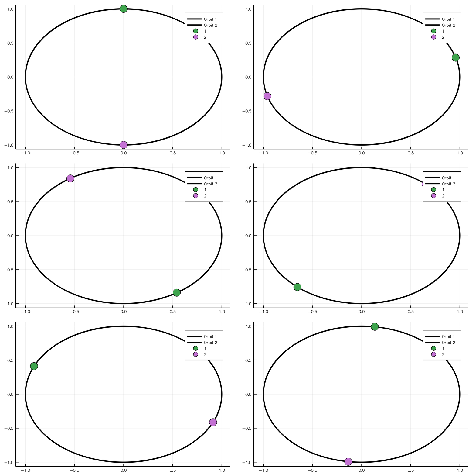

Two bodies rotating on the same orbit

Electrostatic Interaction

Interaction between charged particles obeys Coulomb's law. The movement of such bodies can be simulated using ChargedParticle and ChargedParticles structures. The following example shows how to model two oppositely charged particles. If one body is more massive than another, it will be possible to observe the rotation of the light body around the heavy one without adjusting their positions in space. The constructor for the ChargedParticles system requires bodies and Coulomb's constant k to be passed as arguments.

r = 100.0 # m
q1 = 1e-3 # C
q2 = -1e-3 # C
m1 = 100.0 # kg
m2 = 0.1 # kg
v2 = sqrt(abs(k * q1 * q2 / m2 / r)) # m/s - using the centrifugal acceleration
t = 2 * pi * r / v2 # s  - for one rotation
p1 = ChargedParticle(SVector(0.0, 0.0, 0.0), SVector(0.0, 0, 0.0), m1, q1)
p2 = ChargedParticle(SVector(100.0, 0.0, 0.0), SVector(0.0, v2, 0.0), m2, q2)
system = ChargedParticles([p1, p2], k)
simulation = NBodySimulation(system, (0.0, t))
sim_result = run_simulation(simulation)

Magnetic Interaction

An N-body system consisting of MagneticParticles can be used for the simulation of interacting magnetic dipoles, though such dipoles cannot rotate in space. Such a model can represent single domain particles interacting under the influence of a strong external magnetic field. To create a magnetic particle, one specifies its location in space, velocity, and the vector of its magnetic moment. The following code shows how we can construct an iron particle:

iron_density = 7800 # kg/m^3
magnetization_saturation = 1.2e6 # A/m
mass = 5e-6 # kg
r = SVector(-0.005, 0.0, 0.0) # m
v = SVector(0.0, 0.0, 0.0) # m/s
magnetic_moment = SVector(0.0, 0.0, magnetization_saturation * mass / iron_density) # A*m^2
p1 = MagneticParticle(r, v, mass, magnetic_moment)

For the second particle, we will use a shorter form:

p2 = MagneticParticle(SVector(0.005, 0.0, 0.0), SVector(0.0, 0.0, 0.0), 5e-6,
    SVector(0.0, 0.0, 0.00077))

To calculate magnetic interactions properly, one should also specify the value for the constant μ0/4π or its substitute. Having created parameters for the magnetostatic potential, one can now instantiate a system of particles that should interact magnetically. For that purpose, we use PotentialNBodySystem and pass particles and potential parameters as arguments.

parameters = MagnetostaticParameters(μ_4π)
system = PotentialNBodySystem([p1, p2], Dict(:magnetic => parameters))
simulation = NBodySimulation(system, (t1, t2))
sim_result = run_simulation(simulation, VelocityVerlet(), dt = τ)

Molecular Dynamics (MD)

NBodySimulator allows one to conduct molecular dynamic simulations for the Lennard-Jones liquids, the SPC/Fw model of water, and other molecular systems thanks to implementations of basic interaction potentials between atoms and molecules:

Lennard-Jones
electrostatic and magnetostatic
harmonic bonds
harmonic valence angle generated by pairs of bonds

The comprehensive examples of liquid argon and water simulations can be found in the examples folder. Here only the basic principles of the molecular dynamics simulations using NBodySimulator are presented using liquid argon as a classical MD system for beginners. First, one needs to define the parameters of the simulation:

T = 120.0 # °K
T0 = 90.0 # °K
kb = 8.3144598e-3 # kJ/(K*mol)
ϵ = T * kb
σ = 0.34 # nm
ρ = 1374 / 1.6747# Da/nm^3
m = 39.95# Da
N = 216
L = (m * N / ρ)^(1 / 3)#10.229σ
R = 0.5 * L
v_dev = sqrt(kb * T / m)
bodies = generate_bodies_in_cell_nodes(N, m, v_dev, L)
τ = 0.5e-3 # ps or 1e-12 s
t1 = 0.0
t2 = 2000τ

Liquid argon consists of neutral molecules, so the Lennard-Jones potential governs their interaction:

parameters = LennardJonesParameters(ϵ, σ, R)
lj_system = PotentialNBodySystem(bodies, Dict(:lennard_jones => parameters));

Then, a thermostat and boundary conditions should be selected and instantiated:

thermostat = NoseHooverThermostat(T0, 200τ)
pbc = CubicPeriodicBoundaryConditions(L)
simulation = NBodySimulation(lj_system, (t1, t2), pbc, thermostat, kb);
result = run_simulation(simulation, VelocityVerlet(), dt = τ)

It is recommended to use CubicPeriodicBoundaryConditions since cubic boxes are among the most popular boundary conditions in MD. There are different variants of the NBodySimulation constructor for MD:

simulation = NBodySimulation(lj_system, (t1, t2));
simulation = NBodySimulation(lj_system, (t1, t2), pbc);
simulation = NBodySimulation(lj_system, (t1, t2), pbc, thermostat);
simulation = NBodySimulation(lj_system, (t1, t2), pbc, thermostat, kb);

The default boundary conditions are InfiniteBox without any limits, the default thermostat is NullThermostat (which does no thermostating), and the default Boltzmann constant kb equals its value in SI, i.e., 1.38e-23 J/K.

Water Simulations

In NBodySimulator the SPC/Fw water model is implemented. For using this model, one has to specify parameters of the Lennard-Jones potential between the oxygen atoms of water molecules, parameters of the electrostatic potential for the corresponding interactions between atoms of different molecules, and parameters for harmonic potentials representing bonds between atoms and the valence angle made from bonds between hydrogen atoms and the oxygen atom.

bodies = generate_bodies_in_cell_nodes(N, mH2O, v, L)
jl_parameters = LennardJonesParameters(ϵOO, σOO, R)
e_parameters = ElectrostaticParameters(k, Rel)
spc_parameters = SPCFwParameters(rOH, ∠HOH, k_bond, k_angle)
water = WaterSPCFw(bodies, mH, mO, qH, qO, jl_parameters, e_parameters, spc_parameters);

For each water molecule here, rOH is the equilibrium distance between a hydrogen atom and the oxygen atom, ∠HOH denotes the equilibrium angle made of those two bonds, k_bond and k_angle are the elastic coefficients for the corresponding harmonic potentials. Further, one can pass the water system into the NBodySimulation constructor as a usual system of N-bodies.

simulation = NBodySimulation(water, (t1, t2), pbc, kb);

Thermostats

Usually, during the simulation, a system is required to be at a particular temperature. NBodySimulator contains several thermostats for that purpose. Here the thermostating of liquid argon is presented, for thermostating of water, one can refer to this post.

Andersen Thermostat

τ = 0.5e-3 # timestep of integration and simulation
T0 = 90
ν = 0.05 / τ
thermostat = AndersenThermostat(90, ν)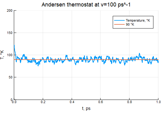

andersen thermostating

Berendsen Thermostat

τB = 2000τ
thermostat = BerendsenThermostat(90, τB)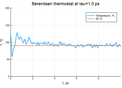

berendsen thermostating

Nosé–Hoover Thermostat

τNH = 200τ
thermostat = NoseHooverThermostat(T0, 200τ)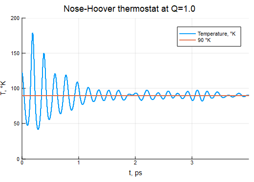

nose-hoover thermostating

Langevin Thermostat

γ = 10.0
thermostat = LangevinThermostat(90, γ)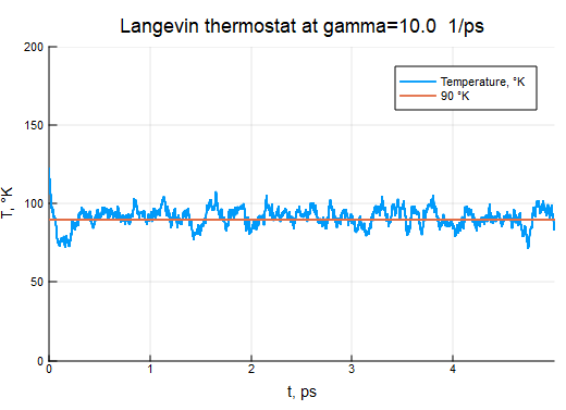

langevin thermostating

Analyzing the Results of the Simulation

Once the simulation is completed, one can analyze the result and obtain some useful characteristics of the system. The function run_simulation returns a structure containing the initial parameters of the simulation and the solution of the differential equation (DE) required for the description of the corresponding system of particles. There are different functions that help to interpret the solution of DEs into physical quantities. One of the main characteristics of a system during molecular dynamics simulations is its thermodynamic temperature. The value of the temperature at a particular time t can be obtained by calling this function:

T = temperature(result, t)

Radial distribution functions

The RDF is another popular and essential characteristic of molecules or similar systems of particles. It shows the reciprocal location of particles averaged by the time of simulation.

(rs, grf) = rdf(result)

The dependence of grf on rs shows the radial distribution of particles at different distances from an average particle in a system. Here, the radial distribution function for the classic system of liquid argon is presented: 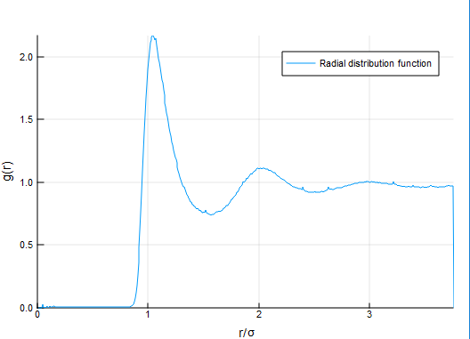rdf for liquid argon

Mean Squared Displacement (MSD)

The MSD characteristic can be used to estimate the shift of particles from their initial positions.

(ts, dr2) = msd(result)

For a standard liquid argon system, the displacement grows with time: 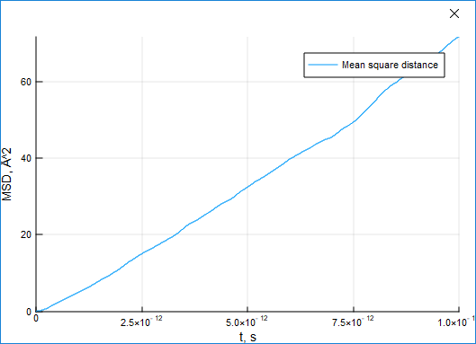rdf for liquid argon

Energy Functions

Energy is a highly important physical characteristic of a system. The module provides four functions to obtain it, though the total_energy function just sums potential and kinetic energy:

e_init = initial_energy(simulation)
e_kin = kinetic_energy(result, t)
e_pot = potential_energy(result, t)
e_tot = total_energy(result, t)

Plotting Images

Using the tools of NBodySimulator, one can export the results of a simulation into a Protein Database File. VMD is a well-known tool for visualizing molecular dynamics, which can read data from PDB files.

save_to_pdb(result, "path_to_a_new_pdb_file.pdb")

In the future, it will be possible to export results via the FileIO interface and its save function. Using Plots.jl, one can draw the positions of particles at any time of simulation or create an animation of moving particles, molecules of water:

using Plots
plot(result)
animate(result, "path_to_file.gif")

Makie.jl also has a recipe for plotting the results of N-body simulations.

Contributing

Please refer to the SciML ColPrac: Contributor's Guide on Collaborative Practices for Community Packages for guidance on PRs, issues, and other matters relating to contributing to SciML.
See the SciML Style Guide for common coding practices and other style decisions.
There are a few community forums:
- The #diffeq-bridged and #sciml-bridged channels in the Julia Slack
- The #diffeq-bridged and #sciml-bridged channels in the Julia Zulip
- On the Julia Discourse forums
- See also SciML Community page

Reproducibility

The documentation of this SciML package was built using these direct dependencies,

Status `~/_work/NBodySimulator.jl/NBodySimulator.jl/docs/Project.toml`
  [e30172f5] Documenter v1.19.0
  [0e6f8da7] NBodySimulator v1.16.0 `~/_work/NBodySimulator.jl/NBodySimulator.jl`

and using this machine and Julia version.

Julia Version 1.13.0
Commit d1c37793dd2 (2026-09-09 19:00 UTC)
Build Info:
  Official https://julialang.org release
Platform Info:
  OS: Linux (x86_64-linux-gnu)
  CPU: 128 × AMD EPYC 7513 32-Core Processor
  WORD_SIZE: 64
  LLVM: libLLVM-20.1.8 (ORCJIT, znver3)
  GC: Built with stock GC
Threads: 1 default, 1 interactive, 1 GC (on 4 virtual cores)
Environment:
  JULIA_CPU_THREADS = 4
  JULIA_NUM_PRECOMPILE_TASKS = 4

A more complete overview of all dependencies and their versions is also provided.

Status `~/_work/NBodySimulator.jl/NBodySimulator.jl/docs/Manifest.toml`
  [47edcb42] ADTypes v1.24.0
  [a4c015fc] ANSIColoredPrinters v0.0.1
  [1520ce14] AbstractTrees v0.4.5
  [7d9f7c33] Accessors v0.1.45
  [79e6a3ab] Adapt v4.7.0
  [4fba245c] ArrayInterface v7.30.1
  [b2a6c25c] BinaryHeaps v1.1.0
  [70df07ce] BracketingNonlinearSolve v1.12.7
  [944b1d66] CodecZlib v0.7.9
  [38540f10] CommonSolve v0.2.14
  [34da2185] Compat v4.18.1
  [a33af91c] CompositionsBase v0.1.2
  [2569d6c7] ConcreteStructs v0.2.8
  [187b0558] ConstructionBase v1.6.0
  [a8cc5b0e] Crayons v4.2.0
  [9a962f9c] DataAPI v1.16.0
  [e2d170a0] DataValueInterfaces v1.0.0
  [2b5f629d] DiffEqBase v7.21.0
  [a0c0ee7d] DifferentiationInterface v0.7.21
  [ffbed154] DocStringExtensions v0.9.5
  [e30172f5] Documenter v1.19.0
  [4e289a0a] EnumX v1.0.7
  [f151be2c] EnzymeCore v0.8.21
  [e2ba6199] ExprTools v0.1.11
  [7034ab61] FastBroadcast v1.4.0
  [9aa1b823] FastClosures v0.3.2
  [a4df4552] FastPower v1.5.0
  [5789e2e9] FileIO v1.20.0
  [64ca27bc] FindFirstFunctions v3.2.1
  [069b7b12] FunctionWrappers v1.1.3
  [77dc65aa] FunctionWrappersWrappers v1.13.0
  [46192b85] GPUArraysCore v0.2.0
  [d7ba0133] Git v1.5.0
  [b5f81e59] IOCapture v1.0.0
  [3587e190] InverseFunctions v0.1.17
  [92d709cd] IrrationalConstants v0.2.6
  [82899510] IteratorInterfaceExtensions v1.0.0
  [692b3bcd] JLLWrappers v1.8.0
  [682c06a0] JSON v1.8.0
  [b964fa9f] LaTeXStrings v1.4.1
  [0e77f7df] LazilyInitializedFields v1.3.0
  [2ab3a3ac] LogExpFunctions v1.0.1
  [e6f89c97] LoggingExtras v1.2.0
  [1914dd2f] MacroTools v0.5.16
  [d0879d2d] MarkdownAST v0.1.3
  [bb5d69b7] MaybeInplace v0.1.8
  [46d2c3a1] MuladdMacro v0.2.7
  [0e6f8da7] NBodySimulator v1.16.0 `~/_work/NBodySimulator.jl/NBodySimulator.jl`
  [be0214bd] NonlinearSolveBase v2.49.5
  [bac558e1] OrderedCollections v2.0.1
  [bbf590c4] OrdinaryDiffEqCore v4.17.0
  [af6ede74] OrdinaryDiffEqRKN v2.2.0
  [fa646aed] OrdinaryDiffEqSymplecticRK v2.2.2
  [b1df2697] OrdinaryDiffEqTsit5 v2.1.4
  [69de0a69] Parsers v3.0.0
  [d236fae5] PreallocationTools v1.7.1
  [aea7be01] PrecompileTools v1.3.4
  [21216c6a] Preferences v1.5.2
  [08abe8d2] PrettyTables v3.4.8
  [3cdcf5f2] RecipesBase v1.3.4
  [731186ca] RecursiveArrayTools v4.5.1
  [189a3867] Reexport v1.2.2
  [2792f1a3] RegistryInstances v0.1.0
  [ae029012] Requires v1.3.1
  [9fe22ead] RespecializeParams v1.3.0
  [7e49a35a] RuntimeGeneratedFunctions v0.5.26
  [0bca4576] SciMLBase v3.53.2
  [19f34311] SciMLJacobianOperators v0.1.19
  [a6db7da4] SciMLLogging v2.1.0
  [c0aeaf25] SciMLOperators v1.30.0
  [431bcebd] SciMLPublic v1.3.0
  [53ae85a6] SciMLStructures v1.10.5
  [efcf1570] Setfield v1.1.2
  [90137ffa] StaticArrays v1.9.20
  [1e83bf80] StaticArraysCore v1.4.4
  [10745b16] Statistics v1.11.5
⌅ [892a3eda] StringManipulation v0.5.0
  [ec057cc2] StructUtils v2.8.5
  [2efcf032] SymbolicIndexingInterface v0.3.55
  [3783bdb8] TableTraits v1.0.1
  [bd369af6] Tables v1.14.0
  [a759f4b9] TimerOutputs v1.2.1
  [3bb67fe8] TranscodingStreams v0.11.3
  [781d530d] TruncatedStacktraces v1.4.0
  [2e619515] Expat_jll v2.8.4+0
  [020c3dae] Git_LFS_jll v3.7.1+0
  [f8c6e375] Git_jll v2.55.0+0
  [94ce4f54] Libiconv_jll v1.18.0+0
  [9bd350c2] OpenSSH_jll v10.5.1+0
  [0dad84c5] ArgTools v1.1.2
  [56f22d72] Artifacts v1.11.0
  [2a0f44e3] Base64 v1.11.0
  [ade2ca70] Dates v1.11.0
  [8ba89e20] Distributed v1.11.0
  [f43a241f] Downloads v1.7.0
  [7b1f6079] FileWatching v1.11.0
  [9fa8497b] Future v1.11.0
  [b77e0a4c] InteractiveUtils v1.11.0
  [ac6e5ff7] JuliaSyntaxHighlighting v1.12.0
  [b27032c2] LibCURL v1.0.0
  [76f85450] LibGit2 v1.11.0
  [8f399da3] Libdl v1.11.0
  [37e2e46d] LinearAlgebra v1.13.0
  [56ddb016] Logging v1.11.0
  [d6f4376e] Markdown v1.11.0
  [ca575930] NetworkOptions v1.3.0
  [44cfe95a] Pkg v1.13.0
  [de0858da] Printf v1.11.0
  [3fa0cd96] REPL v1.11.0
  [9a3f8284] Random v1.11.0
  [ea8e919c] SHA v1.0.0
  [9e88b42a] Serialization v1.11.0
  [6462fe0b] Sockets v1.11.0
  [f489334b] StyledStrings v1.11.0
  [fa267f1f] TOML v1.0.3
  [a4e569a6] Tar v1.10.0
  [8dfed614] Test v1.11.0
  [cf7118a7] UUIDs v1.11.0
  [4ec0a83e] Unicode v1.11.0
  [e66e0078] CompilerSupportLibraries_jll v1.5.5+2
  [deac9b47] LibCURL_jll v8.18.0+1
  [e37daf67] LibGit2_jll v1.9.1+0
  [29816b5a] LibSSH2_jll v1.11.103+0
  [14a3606d] MozillaCACerts_jll v2026.8.13
  [4536629a] OpenBLAS_jll v0.3.30+0
  [458c3c95] OpenSSL_jll v3.5.6+0
  [efcefdf7] PCRE2_jll v10.46.0+0
  [83775a58] Zlib_jll v1.3.1+2
  [3161d3a3] Zstd_jll v1.5.7+1
  [8e850b90] libblastrampoline_jll v5.15.0+0
  [8e850ede] nghttp2_jll v1.67.1+0
  [3f19e933] p7zip_jll v17.8.2+0
Info Packages marked with ⌅ have new versions available but compatibility constraints restrict them from upgrading. To see why use `status --outdated -m`

You can also download the manifest file and the project file.