Transfer Learning with Neural Adapter

Transfer learning is a machine learning technique where a model trained on one task is re-purposed on a second related task.

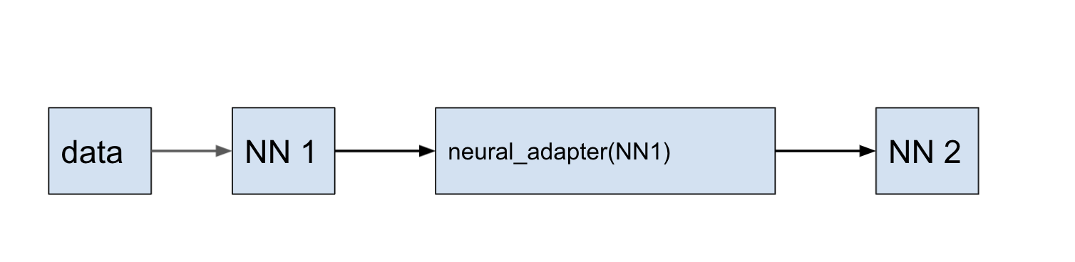
neural_adapter is the method that trains a neural network using the results from an already obtained prediction.

This allows reusing the obtained prediction results and pre-training states of the neural network to get a new prediction, or reuse the results of predictions to train a related task (for example, the same task with a different domain). It makes it possible to create more flexible training schemes.

Retrain the prediction

Using the example of 2D Poisson equation, it is shown how, using the method neural_adapter, to retrain the prediction of one neural network to another.

using NeuralPDE, Lux, ModelingToolkit, Optimization, OptimizationOptimisers
using ModelingToolkit: Interval, infimum, supremum
using Random, ComponentArrays

@parameters x y
@variables u(..)
Dxx = Differential(x)^2
Dyy = Differential(y)^2

# 2D PDE
eq = Dxx(u(x, y)) + Dyy(u(x, y)) ~ -sin(pi * x) * sin(pi * y)

# Initial and boundary conditions
bcs = [u(0, y) ~ 0.0, u(1, y) ~ -sin(pi * 1) * sin(pi * y),
    u(x, 0) ~ 0.0, u(x, 1) ~ -sin(pi * x) * sin(pi * 1)]
# Space and time domains
domains = [x ∈ Interval(0.0, 1.0), y ∈ Interval(0.0, 1.0)]
quadrature_strategy = NeuralPDE.QuadratureTraining(reltol = 1e-3, abstol = 1e-6,
    maxiters = 50, batch = 100)
inner = 8
af = Lux.tanh
chain1 = Lux.Chain(Lux.Dense(2, inner, af),
    Lux.Dense(inner, inner, af),
    Lux.Dense(inner, 1))

discretization = NeuralPDE.PhysicsInformedNN(chain1, quadrature_strategy)

@named pde_system = PDESystem(eq, bcs, domains, [x, y], [u(x, y)])
prob = NeuralPDE.discretize(pde_system, discretization)
sym_prob = NeuralPDE.symbolic_discretize(pde_system, discretization)

callback = function (p, l)
    println("Current loss is: $l")
    return false
end

res = Optimization.solve(prob, OptimizationOptimisers.Adam(5e-3); maxiters = 10000)
phi = discretization.phi

inner_ = 8
af = Lux.tanh
chain2 = Lux.Chain(Dense(2, inner_, af),
    Dense(inner_, inner_, af),
    Dense(inner_, inner_, af),
    Dense(inner_, 1))
initp, st = Lux.setup(Random.default_rng(), chain2)
init_params2 = Float64.(ComponentArrays.ComponentArray(initp))

# the rule by which the training will take place is described here in loss function
function loss(cord, θ)
    global st, chain2
    ch2, st = chain2(cord, θ, st)
    ch2 .- phi(cord, res.u)
end

strategy = NeuralPDE.QuadratureTraining(; reltol = 1e-6, abstol = 1e-3)

prob_ = NeuralPDE.neural_adapter(loss, init_params2, pde_system, strategy)
res_ = Optimization.solve(prob_, OptimizationOptimisers.Adam(5e-3); maxiters = 10000)

phi_ = PhysicsInformedNN(chain2, strategy; init_params = res_.u).phi

xs, ys = [infimum(d.domain):0.01:supremum(d.domain) for d in domains]
analytic_sol_func(x, y) = (sin(pi * x) * sin(pi * y)) / (2pi^2)

u_predict = reshape([first(phi([x, y], res.u)) for x in xs for y in ys],
    (length(xs), length(ys)))
u_predict_ = reshape([first(phi_([x, y], res_.u)) for x in xs for y in ys],
    (length(xs), length(ys)))
u_real = reshape([analytic_sol_func(x, y) for x in xs for y in ys],
    (length(xs), length(ys)))
diff_u = u_predict .- u_real
diff_u_ = u_predict_ .- u_real

using Plots
p1 = plot(xs, ys, u_predict, linetype = :contourf, title = "first predict")
p2 = plot(xs, ys, u_predict_, linetype = :contourf, title = "second predict")
p3 = plot(xs, ys, u_real, linetype = :contourf, title = "analytic")
p4 = plot(xs, ys, diff_u, linetype = :contourf, title = "error 1")
p5 = plot(xs, ys, diff_u_, linetype = :contourf, title = "error 2")
plot(p1, p2, p3, p4, p5)

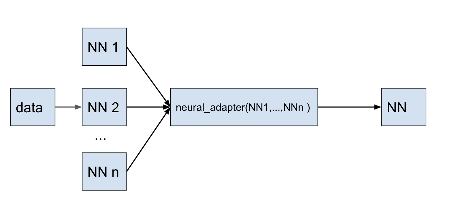
Domain decomposition

In this example, we first obtain a prediction of 2D Poisson equation on subdomains. We split up full domain into 10 sub problems by x, and create separate neural networks for each sub interval. If x domain ∈ [x0, xend] so, it is decomposed on 10 part: sub x domains = {[x0, x1], ... [xi,xi+1], ..., x9,xend]}. And then using the method neural_adapter, we retrain the batch of 10 predictions to the one prediction for full domain of task.

using NeuralPDE, Lux, ModelingToolkit, Optimization, OptimizationOptimisers
using ModelingToolkit: Interval, infimum, supremum

@parameters x y
@variables u(..)
Dxx = Differential(x)^2
Dyy = Differential(y)^2

eq = Dxx(u(x, y)) + Dyy(u(x, y)) ~ -sin(pi * x) * sin(pi * y)

bcs = [u(0, y) ~ 0.0, u(1, y) ~ -sin(pi * 1) * sin(pi * y),
    u(x, 0) ~ 0.0, u(x, 1) ~ -sin(pi * x) * sin(pi * 1)]

# Space
x_0 = 0.0
x_end = 1.0
x_domain = Interval(x_0, x_end)
y_domain = Interval(0.0, 1.0)
domains = [x ∈ x_domain, y ∈ y_domain]

count_decomp = 10

# Neural network
af = Lux.tanh
inner = 10
chains = [Lux.Chain(Dense(2, inner, af), Dense(inner, inner, af), Dense(inner, 1))
          for _ in 1:count_decomp]
init_params = map(
    c -> Float64.(ComponentArray(Lux.setup(Random.default_rng(), c)[1])), chains)

xs_ = infimum(x_domain):(1 / count_decomp):supremum(x_domain)
xs_domain = [(xs_[i], xs_[i + 1]) for i in 1:(length(xs_) - 1)]
domains_map = map(xs_domain) do (xs_dom)
    x_domain_ = Interval(xs_dom...)
    domains_ = [x ∈ x_domain_,
        y ∈ y_domain]
end

analytic_sol_func(x, y) = (sin(pi * x) * sin(pi * y)) / (2pi^2)
function create_bcs(x_domain_, phi_bound)
    x_0, x_e = x_domain_.left, x_domain_.right
    if x_0 == 0.0
        bcs = [u(0, y) ~ 0.0,
            u(x_e, y) ~ analytic_sol_func(x_e, y),
            u(x, 0) ~ 0.0,
            u(x, 1) ~ -sin(pi * x) * sin(pi * 1)]
        return bcs
    end
    bcs = [u(x_0, y) ~ phi_bound(x_0, y),
        u(x_e, y) ~ analytic_sol_func(x_e, y),
        u(x, 0) ~ 0.0,
        u(x, 1) ~ -sin(pi * x) * sin(pi * 1)]
    bcs
end

reses = []
phis = []
pde_system_map = []

for i in 1:count_decomp
    println("decomposition $i")
    domains_ = domains_map[i]
    phi_in(cord) = phis[i - 1](cord, reses[i - 1].u)
    phi_bound(x, y) = phi_in(vcat(x, y))
    @register_symbolic phi_bound(x, y)
    Base.Broadcast.broadcasted(::typeof(phi_bound), x, y) = phi_bound(x, y)
    bcs_ = create_bcs(domains_[1].domain, phi_bound)
    @named pde_system_ = PDESystem(eq, bcs_, domains_, [x, y], [u(x, y)])
    push!(pde_system_map, pde_system_)
    strategy = NeuralPDE.QuadratureTraining(; reltol = 1e-6, abstol = 1e-3)

    discretization = NeuralPDE.PhysicsInformedNN(chains[i], strategy;
        init_params = init_params[i])

    prob = NeuralPDE.discretize(pde_system_, discretization)
    symprob = NeuralPDE.symbolic_discretize(pde_system_, discretization)
    res_ = Optimization.solve(prob, OptimizationOptimisers.Adam(5e-3); maxiters = 10000)
    phi = discretization.phi
    push!(reses, res_)
    push!(phis, phi)
end

function compose_result(dx)
    u_predict_array = Float64[]
    diff_u_array = Float64[]
    ys = infimum(domains[2].domain):dx:supremum(domains[2].domain)
    xs_ = infimum(x_domain):dx:supremum(x_domain)
    xs = collect(xs_)
    function index_of_interval(x_)
        for (i, x_domain) in enumerate(xs_domain)
            if x_ <= x_domain[2] && x_ >= x_domain[1]
                return i
            end
        end
    end
    for x_ in xs
        i = index_of_interval(x_)
        u_predict_sub = [first(phis[i]([x_, y], reses[i].u)) for y in ys]
        u_real_sub = [analytic_sol_func(x_, y) for y in ys]
        diff_u_sub = abs.(u_predict_sub .- u_real_sub)
        append!(u_predict_array, u_predict_sub)
        append!(diff_u_array, diff_u_sub)
    end
    xs, ys = [infimum(d.domain):dx:supremum(d.domain) for d in domains]
    u_predict = reshape(u_predict_array, (length(xs), length(ys)))
    diff_u = reshape(diff_u_array, (length(xs), length(ys)))
    u_predict, diff_u
end

dx = 0.01
u_predict, diff_u = compose_result(dx)

inner_ = 18
af = Lux.tanh
chain2 = Lux.Chain(Dense(2, inner_, af),
    Dense(inner_, inner_, af),
    Dense(inner_, inner_, af),
    Dense(inner_, inner_, af),
    Dense(inner_, 1))

initp, st = Lux.setup(Random.default_rng(), chain2)
init_params2 = Float64.(ComponentArrays.ComponentArray(initp))

@named pde_system = PDESystem(eq, bcs, domains, [x, y], [u(x, y)])

losses = map(1:count_decomp) do i
    function loss(cord, θ)
        global st, chain2, phis, reses
        ch2, st = chain2(cord, θ, st)
        ch2 .- phis[i](cord, reses[i].u)
    end
end

callback = function (p, l)
    println("Current loss is: $l")
    return false
end

prob_ = NeuralPDE.neural_adapter(losses, init_params2, pde_system_map,
    NeuralPDE.QuadratureTraining(; reltol = 1e-6, abstol = 1e-3))
res_ = Optimization.solve(prob_, OptimizationOptimisers.Adam(5e-3); maxiters = 5000)
prob_ = NeuralPDE.neural_adapter(losses, res_.u, pde_system_map,
    NeuralPDE.QuadratureTraining(; reltol = 1e-6, abstol = 1e-3))
res_ = Optimization.solve(prob_, OptimizationOptimisers.Adam(5e-3); maxiters = 5000)

phi_ = PhysicsInformedNN(chain2, strategy; init_params = res_.u).phi

xs, ys = [infimum(d.domain):dx:supremum(d.domain) for d in domains]
u_predict_ = reshape([first(phi_([x, y], res_.u)) for x in xs for y in ys],
    (length(xs), length(ys)))
u_real = reshape([analytic_sol_func(x, y) for x in xs for y in ys],
    (length(xs), length(ys)))
diff_u_ = u_predict_ .- u_real

using Plots

p1 = plot(xs, ys, u_predict, linetype = :contourf, title = "predict 1");
p2 = plot(xs, ys, u_predict_, linetype = :contourf, title = "predict 2");
p3 = plot(xs, ys, u_real, linetype = :contourf, title = "analytic");
p4 = plot(xs, ys, diff_u, linetype = :contourf, title = "error 1");
p5 = plot(xs, ys, diff_u_, linetype = :contourf, title = "error 2");
plot(p1, p2, p3, p4, p5)