Physics-Informed Neural Networks solver

Example 1: Solving the 2-dimensional Poisson Equation

In this example, we will solve a Poisson equation of 2 dimensions:

with the boundary conditions:

on the space domain:

with grid discretization dx = 0.1.

The ModelingToolkit PDE interface for this example looks like this:

using NeuralPDE, Flux, ModelingToolkit, GalacticOptim, Optim, DiffEqFlux
@parameters x y
@variables u(..)
@derivatives Dxx''~x
@derivatives Dyy''~y

# 2D PDE
eq  = Dxx(u(x,y)) + Dyy(u(x,y)) ~ -sin(pi*x)*sin(pi*y)

# Boundary conditions
bcs = [u(0,y) ~ 0.f0, u(1,y) ~ -sin(pi*1)*sin(pi*y),
       u(x,0) ~ 0.f0, u(x,1) ~ -sin(pi*x)*sin(pi*1)]
# Space and time domains
domains = [x ∈ IntervalDomain(0.0,1.0),
           y ∈ IntervalDomain(0.0,1.0)]

Here, we define the neural network, where the input of NN equals the number of dimensions and output equals the number of equations in the system.

# Neural network
dim = 2 # number of dimensions
chain = FastChain(FastDense(dim,16,Flux.σ),FastDense(16,16,Flux.σ),FastDense(16,1))

Here, we build PhysicsInformedNN algorithm where dx is the step of discretization and strategy stores information for choosing a training strategy.

# Discretization
dx = 0.05
discretization = PhysicsInformedNN(dx,
                                   chain,
                                   strategy = GridTraining())

As described in the API docs, we now need to define the PDESystem and create PINNs problem using the discretize method.

pde_system = PDESystem(eq,bcs,domains,[x,y],[u])
prob = discretize(pde_system,discretization)

Here, we define the callback function and the optimizer. And now we can solve the PDE using PINNs (with the number of epochs maxiters=1000).

cb = function (p,l)
    println("Current loss is: $l")
    return false
end

res = GalacticOptim.solve(prob, BFGS(), progress = false; cb = cb, maxiters=1000)
phi = discretization.phi

We can plot the predicted solution of the PDE and compare it with the analytical solution in order to plot the relative error.

xs,ys = [domain.domain.lower:dx/10:domain.domain.upper for domain in domains]
analytic_sol_func(x,y) = (sin(pi*x)*sin(pi*y))/(2pi^2)

u_predict = reshape([first(phi([x,y],res.minimizer)) for x in xs for y in ys],(length(xs),length(ys)))
u_real = reshape([analytic_sol_func(x,y) for x in xs for y in ys], (length(xs),length(ys)))
diff_u = abs.(u_predict .- u_real)

p1 = plot(xs, ys, u_real, linetype=:contourf,title = "analytic");
p2 = plot(xs, ys, u_predict, linetype=:contourf,title = "predict");
p3 = plot(xs, ys, diff_u,linetype=:contourf,title = "error");
plot(p1,p2,p3)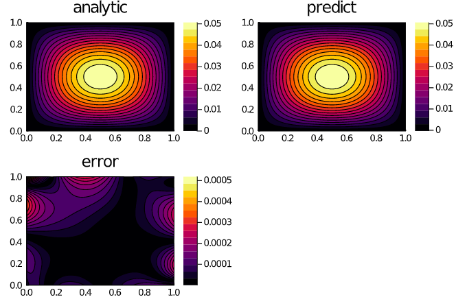

Example 2 : Solving the 2-dimensional Wave Equation with Neumann boundary condition

Let's solve this 2-dimensional wave equation:

with grid discretization dx = 0.1.

Further, the solution of this equation with the given boundary conditions is presented.

@parameters x, t
@variables u(..)
@derivatives Dxx''~x
@derivatives Dtt''~t
@derivatives Dt'~t

#2D PDE
C=1
eq  = Dtt(u(x,t)) ~ C^2*Dxx(u(x,t))

# Initial and boundary conditions
bcs = [u(0,t) ~ 0.,# for all t > 0
       u(1,t) ~ 0.,# for all t > 0
       u(x,0) ~ x*(1. - x), #for all 0 < x < 1
       Dt(u(x,0)) ~ 0. ] #for all  0 < x < 1]

# Space and time domains
domains = [x ∈ IntervalDomain(0.0,1.0),
           t ∈ IntervalDomain(0.0,1.0)]
# Discretization
dx = 0.1

# Neural network
chain = FastChain(FastDense(2,16,Flux.σ),FastDense(16,16,Flux.σ),FastDense(16,1))

discretization = PhysicsInformedNN(dx,
                                   chain,
                                   strategy= GridTraining())

pde_system = PDESystem(eq,bcs,domains,[x,t],[u])
prob = discretize(pde_system,discretization)

# optimizer
opt = Optim.BFGS()
res = GalacticOptim.solve(prob,opt; cb = cb, maxiters=1200)
phi = discretization.phi

We can plot the predicted solution of the PDE and compare it with the analytical solution in order to plot the relative error.

xs,ts = [domain.domain.lower:dx:domain.domain.upper for domain in domains]
analytic_sol_func(x,t) =  sum([(8/(k^3*pi^3)) * sin(k*pi*x)*cos(C*k*pi*t) for k in 1:2:50000])

u_predict = reshape([first(phi([x,t],res.minimizer)) for x in xs for t in ts],(length(xs),length(ts)))
u_real = reshape([analytic_sol_func(x,t) for x in xs for t in ts], (length(xs),length(ts)))

diff_u = abs.(u_predict .- u_real)
p1 = plot(xs, ts, u_real, linetype=:contourf,title = "analytic");
p2 =plot(xs, ts, u_predict, linetype=:contourf,title = "predict");
p3 = plot(xs, ts, diff_u,linetype=:contourf,title = "error");
plot(p1,p2,p3)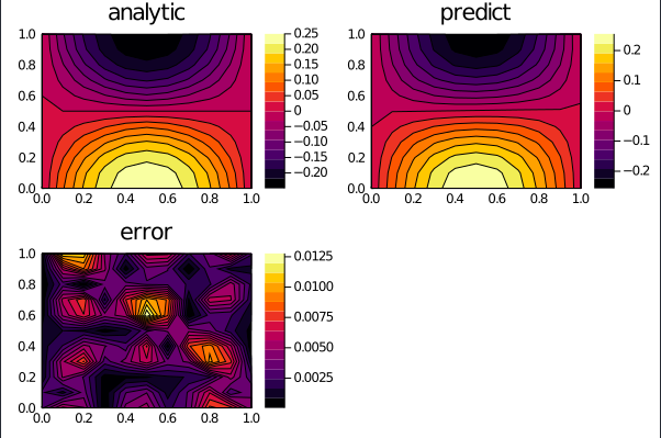

Example 3 : Solving the 3-dimensional PDE

the 3-dimensional PDE:

with the initial and boundary conditions:

on the space and time domain:

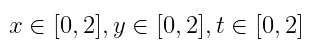
with grid discretization dx = 0.25, dy = 0.25, dt = 0.25.

# 3D PDE
@parameters x y t
@variables u(..)
@derivatives Dxx''~x
@derivatives Dyy''~y
@derivatives Dt'~t

# 3D PDE
eq  = Dt(u(x,y,t)) ~ Dxx(u(x,y,t)) + Dyy(u(x,y,t))
# Initial and boundary conditions
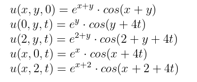
bcs = [u(x,y,0) ~ exp(x+y)*cos(x+y) ,
       u(0,y,t) ~ exp(y)*cos(y+4t)
       u(2,y,t) ~ exp(2+y)*cos(2+y+4t) ,
       u(x,0,t) ~ exp(x)*cos(x+4t),
       u(x,2,t) ~ exp(x+2)*cos(x+2+4t)]
# Space and time domains
domains = [x ∈ IntervalDomain(0.0,2.0),
           y ∈ IntervalDomain(0.0,2.0),
           t ∈ IntervalDomain(0.0,2.0)]

# Discretization
dx = 0.25; dy= 0.25; dt = 0.25
# Neural network
chain = FastChain(FastDense(3,16,Flux.σ),FastDense(16,16,Flux.σ),FastDense(16,1))

discretization = NeuralPDE.PhysicsInformedNN([dx,dy,dt],
                                             chain,
                                             strategy = NeuralPDE.StochasticTraining(include_frac=0.9))
pde_system = PDESystem(eq,bcs,domains,[x,y,t],[u])
prob = NeuralPDE.discretize(pde_system,discretization)

res = GalacticOptim.solve(prob, ADAM(0.1), progress = false; cb = cb, maxiters=3000)
phi = discretization.phi

Example 4 : Solving a PDE System

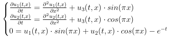
In this example, we will solve the PDE system:

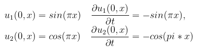
with the initial conditions:

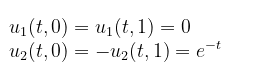
and the boundary conditions:

@parameters t, x
@variables u1(..), u2(..), u3(..)
@derivatives Dt'~t
@derivatives Dtt''~t
@derivatives Dx'~x
@derivatives Dxx''~x

eqs = [Dtt(u1(t,x)) ~ Dxx(u1(t,x)) + u3(t,x)*sin(pi*x),
       Dtt(u2(t,x)) ~ Dxx(u2(t,x)) + u3(t,x)*cos(pi*x),
       0. ~ u1(t,x)*sin(pi*x) + u2(t,x)*cos(pi*x) - exp(-t)]

bcs = [u1(0,x) ~ sin(pi*x),
       u2(0,x) ~ cos(pi*x),
       Dt(u1(0,x)) ~ -sin(pi*x),
       Dt(u2(0,x)) ~ -cos(pi*x),
       u1(t,0) ~ 0.,
       u2(t,0) ~ exp(-t),
       u1(t,1) ~ 0.,
       u2(t,1) ~ -exp(-t),
       u1(t,0) ~ u1(t,1),
       u2(t,0) ~ -u2(t,1)]


# Space and time domains
domains = [t ∈ IntervalDomain(0.0,1.0),
           x ∈ IntervalDomain(0.0,1.0)]
# Discretization
dx = 0.1
# Neural network
input_ = length(domains)
output = length(eqs)
chain = FastChain(FastDense(input_,16,Flux.σ),FastDense(16,16,Flux.σ),FastDense(16,output))

strategy = GridTraining()
discretization = PhysicsInformedNN(dx,chain,strategy=strategy)

pde_system = PDESystem(eqs,bcs,domains,[t,x],[u1,u2,u3])
prob = discretize(pde_system,discretization)

res = GalacticOptim.solve(prob,Optim.BFGS(); cb = cb, maxiters=2000)
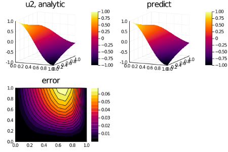
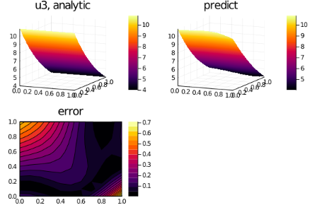
phi = discretization.phi

And some analysis:

ts,xs = [domain.domain.lower:dx:domain.domain.upper for domain in domains]

analytic_sol_func(t,x) = [exp(-t)*sin(pi*x), exp(-t)*cos(pi*x), (1+pi^2)*exp(-t)]
u_real  = [[analytic_sol_func(t,x)[i] for t in ts for x in xs] for i in 1:3]
u_predict  = [[phi([t,x],res.minimizer)[i] for t in ts for x in xs] for i in 1:3]
diff_u = [abs.(u_real[i] .- u_predict[i] ) for i in 1:3]

for i in 1:3
    p1 = plot(xs, ts, u_real[i], st=:surface,title = "u$i, analytic");
    p2 = plot(xs, ts, u_predict[i], st=:surface,title = "predict");
    p3 = plot(xs, ts, diff_u[i],linetype=:contourf,title = "error");
    plot(p1,p2,p3)
    savefig("sol_u$i")
end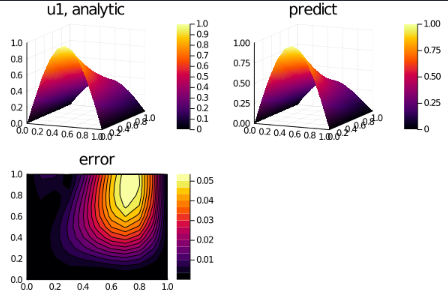

Matrix PDEs form

Also, in addition to systems, we can use the matrix form of PDEs:

@parameters x y
@variables u[1:2,1:2](..)
@derivatives Dxx''~x
@derivatives Dyy''~y

# matrix PDE
eqs  = @. [(Dxx(u_(x,y)) + Dyy(u_(x,y))) for u_ in u] ~ -sin(pi*x)*sin(pi*y)*[0 1; 0 1]

# Initial and boundary conditions
bcs = [u[1](x,0) ~ x, u[2](x,0) ~ 2, u[3](x,0) ~ 3, u[4](x,0) ~ 4]

Example 5 : Solving an ODE with a 3rd-order derivative

Let's consider the ODE with a 3rd-order derivative:

with grid discretization dx = 0.1.

@parameters x
@variables u(..)
@derivatives Dxxx'''~x
@derivatives Dx'~x

# ODE
eq = Dxxx(u(x)) ~ cos(pi*x)

# Initial and boundary conditions
bcs = [u(0.) ~ 0.0,
       u(1.) ~ cos(pi),
       Dx(u(1.)) ~ 1.0]

# Space and time domains
domains = [x ∈ IntervalDomain(0.0,1.0)]

# Discretization
dx = 0.05

# Neural network
chain = FastChain(FastDense(1,8,Flux.σ),FastDense(8,1))

discretization = PhysicsInformedNN(dx,
                                   chain,
                                   strategy=StochasticTraining(include_frac=0.5))
pde_system = PDESystem(eq,bcs,domains,[x],[u])
prob = discretize(pde_system,discretization)

res = GalacticOptim.solve(prob, ADAM(0.01), progress = false; cb = cb, maxiters=2000)
phi = discretization.phi

We can plot the predicted solution of the ODE and its analytical solution.

analytic_sol_func(x) = (π*x*(-x+(π^2)*(2*x-3)+1)-sin(π*x))/(π^3)

xs = [domain.domain.lower:dx/10:domain.domain.upper for domain in domains][1]
u_real  = [analytic_sol_func(x) for x in xs]
u_predict  = [first(phi(x,res.minimizer)) for x in xs]

x_plot = collect(xs)
plot(x_plot ,u_real,title = "real")
plot!(x_plot ,u_predict,title = "predict")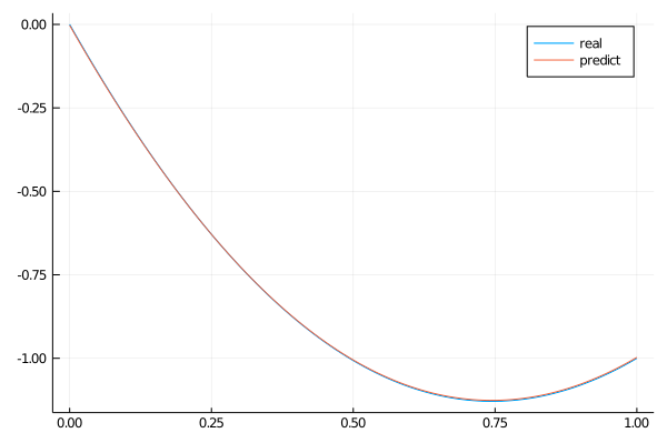

Example 6 : 2-D Burgers' equation, low-level API

Let's consider the Burgers’ equation:

Here is an example of using the low-level API:

@parameters t, x
@variables u(..)
@derivatives Dt'~t
@derivatives Dx'~x
@derivatives Dxx''~x

#2D PDE
eq  = Dt(u(t,x)) + u(t,x)*Dx(u(t,x)) - (0.01/pi)*Dxx(u(t,x)) ~ 0

# Initial and boundary conditions
bcs = [u(0,x) ~ -sin(pi*x),
       u(t,-1) ~ 0.,
       u(t,1) ~ 0.]

# Space and time domains
domains = [t ∈ IntervalDomain(0.0,1.0),
           x ∈ IntervalDomain(-1.0,1.0)]
# Discretization
dx = 0.1
# Neural network
chain = FastChain(FastDense(2,16,Flux.σ),FastDense(16,16,Flux.σ),FastDense(16,1))

strategy = GridTraining()
discretization = PhysicsInformedNN(dx,chain,strategy=strategy)

indvars = [t,x]
depvars = [u]
dim = length(domains)

expr_pde_loss_function = build_loss_function(eq,indvars,depvars)
expr_bc_loss_functions = [build_loss_function(bc,indvars,depvars) for bc in bcs]

train_sets = generate_training_sets(domains,dx,bcs,indvars,depvars)
train_domain_set, train_bound_set, train_set= train_sets

phi = discretization.phi
autodiff = discretization.autodiff
derivative = discretization.derivative
initθ = discretization.initθ

pde_loss_function = get_loss_function(eval(expr_pde_loss_function),
                                      train_domain_set,
                                      phi,
                                      derivative,
                                      strategy)
bc_loss_function = get_loss_function(eval.(expr_bc_loss_functions),
                                     train_bound_set,
                                     phi,
                                     derivative,
                                     strategy)

function loss_function(θ,p)
    return pde_loss_function(θ) + bc_loss_function(θ)
end
f = OptimizationFunction(loss_function, GalacticOptim.AutoZygote())
prob = GalacticOptim.OptimizationProblem(f, initθ)

# optimizer
opt = Optim.BFGS()
res = GalacticOptim.solve(prob, opt; cb = cb, maxiters=1500)
phi = discretization.phi

And some analysis:

ts,xs = [domain.domain.lower:dx:domain.domain.upper for domain in domains]
u_predict_contourf = reshape([first(phi([t,x],res.minimizer)) for t in ts for x in xs] ,length(xs),length(ts))
plot(ts, xs, u_predict_contourf, linetype=:contourf,title = "predict")

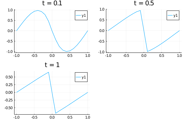
u_predict = [[first(phi([t,x],res.minimizer)) for x in xs] for t in ts ]
p1= plot(xs, u_predict[2],title = "t = 0.1");
p2= plot(xs, u_predict[6],title = "t = 0.5");
p3= plot(xs, u_predict[end],title = "t = 1");
plot(p1,p2,p3)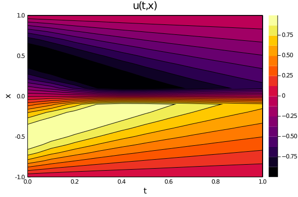

Example 7 : Kuramoto–Sivashinsky equation

Let's consider the Kuramoto–Sivashinsky equation, which contains a 4th-order derivative:

with the initial and boundary conditions:

@parameters x, t
@variables u(..)
@derivatives Dt'~t
@derivatives Dx'~x
@derivatives Dx2''~x
@derivatives Dx3'''~x
@derivatives Dx4''''~x

α = 1
β = 4
γ = 1
eq = Dt(u(x,t)) + u(x,t)*Dx(u(x,t)) + α*Dx2(u(x,t)) + β*Dx3(u(x,t)) + γ*Dx4(u(x,t)) ~ 0

u_analytic(x,t;z = -x/2+t) = 11 + 15*tanh(z) -15*tanh(z)^2 - 15*tanh(z)^3
du(x,t;z = -x/2+t) = 15/2*(tanh(z) + 1)*(3*tanh(z) - 1)*sech(z)^2

bcs = [u(x,0) ~ u_analytic(x,0),
       u(-10,t) ~ u_analytic(-10,t),
       u(10,t) ~ u_analytic(10,t),
       Dx(u(-10,t)) ~ du(-10,t),
       Dx(u(10,t)) ~ du(10,t)]

# Space and time domains
domains = [x ∈ IntervalDomain(-10.0,10.0),
           t ∈ IntervalDomain(0.0,1.0)]
# Discretization
dx = 0.4; dt = 0.2

# Neural network
chain = FastChain(FastDense(2,12,Flux.σ),FastDense(12,12,Flux.σ),FastDense(12,1))

discretization = PhysicsInformedNN([dx,dt],
                                    chain,
                                    strategy = GridTraining())
pde_system = PDESystem(eq,bcs,domains,[x,t],[u])
prob = discretize(pde_system,discretization)

opt = Optim.BFGS()
res = GalacticOptim.solve(prob,opt; cb = cb, maxiters=2000)
phi = discretization.phi

And some analysis:

xs,ts = [domain.domain.lower:dx:domain.domain.upper for (domain,dx) in zip(domains,[dx/10,dt])]

u_predict = [[first(phi([x,t],res.minimizer)) for x in xs] for t in ts]
u_real = [[u_analytic(x,t) for x in xs] for t in ts]
diff_u = [[abs(u_analytic(x,t) -first(phi([x,t],res.minimizer)))  for x in xs] for t in ts]

p1 =plot(xs,u_predict,title = "predict")
p2 =plot(xs,u_real,title = "analytic")
p3 =plot(xs,diff_u,title = "error")
plot(p1,p2,p3)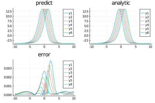

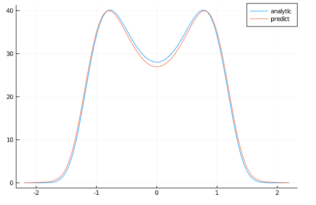
Example 8 : Fokker-Planck equation

Let's consider the Fokker-Planck equation:

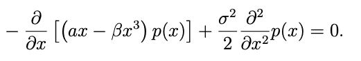
which must satisfy the normalization condition:

with the boundary conditions:

# the example is taken from this article https://arxiv.org/abs/1910.10503
@parameters x
@variables p(..)
@derivatives Dx'~x
@derivatives Dxx''~x

#2D PDE
α = 0.3
β = 0.5
_σ = 0.5
# Discretization
dx = 0.05
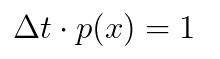
# here we use normalization condition: dx*p(x) ~ 1 in order to get a non-zero solution.
eq  = [(α - 3*β*x^2)*p(x) + (α*x - β*x^3)*Dx(p(x)) ~ (_σ^2/2)*Dxx(p(x)),
       dx*p(x) ~ 1.]

# Initial and boundary conditions
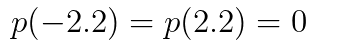
bcs = [p(-2.2) ~ 0. ,p(2.2) ~ 0. , p(-2.2) ~ p(2.2)]

# Space and time domains
domains = [x ∈ IntervalDomain(-2.2,2.2)]

# Neural network
chain = FastChain(FastDense(1,12,Flux.σ),FastDense(12,12,Flux.σ),FastDense(12,1))

discretization = NeuralPDE.PhysicsInformedNN(dx,
                                             chain,
                                             strategy= NeuralPDE.GridTraining())

pde_system = PDESystem(eq,bcs,domains,[x],[p])
prob = NeuralPDE.discretize(pde_system,discretization)

res = GalacticOptim.solve(prob, BFGS(); cb = cb, maxiters=8000)
phi = discretization.phi

And some analysis:

analytic_sol_func(x) = 28.022*exp((1/(2*_σ^2))*(2*α*x^2 - β*x^4))

xs = [domain.domain.lower:dx:domain.domain.upper for domain in domains][1]
u_real  = [analytic_sol_func(x) for x in xs]
u_predict  = [first(phi(x,res.minimizer)) for x in xs]

plot(xs ,u_real, label = "analytic")
plot!(xs ,u_predict, label = "predict")