Physics-Informed Neural Networks

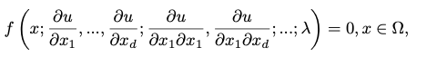
Using the PINNs solver, we can solve general nonlinear PDEs:

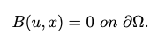
with suitable boundary conditions:

where time t is a special component of x, and Ω contains the temporal domain.

We describe the PDE in the form of the ModelingToolKit interface. See an example of how this can be done above or take a look at the tests.

A General PDE Problem can be defined using a PDESystem:

pde_system = PDESystem(eq,bcs,domains,param,var)

Here, eq is the equation, bcs represents the boundary conditions, param is the parameter of the equation (like [x,y]), and var represents variables (like [u]).

To solve this problem, use the PhysicsInformedNN algorithm.

discretization = PhysicsInformedNN(chain,
                                   nothing; #init_params
                                   phi = nothing,
                                   derivative = nothing,
                                   strategy = GridTraining())

Here,

• chain is a Flux.jl chain, where the input of NN equals the number of dimensions and output equals the number of equations in the system
• init_params is the initial parameter of the neural network
• phi is a trial solution
• derivative is a method that calculates the derivative
• strategy determines which training strategy will be used.

The method discretize interprets from the ModelingToolkit PDE form to the PINNs Problem.

prob = discretize(pde_system, discretization)

To run solve, we can use:

res = GalacticOptim.solve(prob, opt;  cb = cb, maxiters=maxiters)

Here, opt is an optimizer, cb is a callback function, and maxiters is a number of iterations.

Training strategy

List of training strategies that are available now:

• GridTraining(): Initialize points on a lattice and never change them during

the training process.

• StochasticTraining(): In each optimization iteration, we randomly select

the subset of points from a full training set.

• QuasiRandomTraining(): The training set is generated on [Quasi-Monte Carlo

samples](https://github.com/SciML/QuasiMonteCarlo.jl)

• QuadratureTraining(): Сompute an approximation of the integral of the loss function at each iteration using adaptive quadrature methods.

The following algorithms are available: CubaVegas, CubaSUAVE, CubaDivonne,HCubatureJL, CubatureJLh, CubatureJLp, CubaCuhre

More details, about the implementation of the algorithms used, can be found in Quadrature.jl

Low-level API

Besides the high-level API: discretize(pde_system, discretization), we can also use the low-level API methods: build_loss_function, get_loss_function,generate_training_sets, get_phi, get_numeric_derivative, build_symbolic_loss_function, symbolic_discretize.

See how this can be used in the docs examples or take a look at the tests.