Randomization methods
Most of the methods presented in Sampler are deterministic, i.e. X = sample(n, d, ::DeterministicSamplingAlgorithm) will always produce the same sequence $X = (X_1, \dots, X_n)$.
The main issue with deterministic Quasi Monte Carlo sampling is that it does not allow easy error estimation as opposed to plain Monte Carlo, where the variance can be estimated.
A Randomized Quasi Monte Carlo method must respect the two following criteria:
- Have $X_i\sim \mathbb{U}([0,1]^d)$ for each $i\in \{1,\cdots, n\}$.
- Preserve the QMC properties, i.e. the randomized $X$ still has low discrepancy.
This randomized version is unbiased and can be used to obtain a confidence interval or to do sensitivity analysis.
A good reference is the book by A. Owen, especially the Chapters 15, 16 and 17.
API for randomization
QuasiMonteCarlo.RandomizationMethod — Type
RandomizationMethodAbstract interface for methods that randomize deterministic point sets with randomize.
An implementation must preserve the shape of its input point matrix and keep every point in the unit box. It should provide randomize(points::AbstractMatrix, method) and return a new matrix unless the method is explicitly documented as mutating its input. The randomization must preserve the low-discrepancy properties promised by the concrete method and should use an owned or supplied random-number generator for reproducibility.
Deterministic samplers store their default randomization method in an R field. Pass a method explicitly to randomize when a different randomization is needed for an existing point set.
There are two ways to obtain a randomized sequence:
- Either directly use
QuasiMonteCarlo.sample(n, d, DeterministicSamplingAlgorithm(R = SomeRandomizationMethod()))orsample(n, lb, up, DeterministicSamplingAlgorithm(R = RandomizationMethod())). - Or, given $n$ points $d$-dimensional points, all in $[0,1]^d$ one can do
randomize(X, SomeRandomizationMethod())where $X$ is a $d\times n$-matrix.
QuasiMonteCarlo.randomize — Function
randomize(x, R::RandomizationMethod)Apply the randomization method R to a sample matrix x.
Arguments
x::AbstractMatrix: Matrix with one point per column. Its entries must be in the unit box expected by the selected randomization method.R::RandomizationMethod: Randomization strategy to apply.
Returns
- A matrix with the same size as
x, with each point randomized according toR.NoRand()returns the original matrix unchanged; other methods return a new matrix unless their method documentation says otherwise.
Examples
julia> using QuasiMonteCarlo

julia> points = sample(4, 2, SobolSample());

julia> randomized = randomize(points, Shift());

julia> size(randomized) == size(points)
trueThe default method of DeterministicSamplingAlgorithm is NoRand
QuasiMonteCarlo.NoRand — Type
NoRand() <: RandomizationMethodIdentity randomization for deterministic samplers.
randomize(points, NoRand()) returns points unchanged. It is also the default value of the R field on deterministic sampler types.
Examples
julia> using QuasiMonteCarlo

julia> points = sample(4, 2, SobolSample(R = NoRand()));

julia> randomize(points, NoRand()) === points
trueTo obtain multiple independent randomizations of a sequence, i.e. Design Matrices, look at the Design Matrices section.
In most other QMC packages, randomization is performed "online" as the points are samples. Here, randomization is performed after the deterministic sequence is generated. Both methods are useful in different contexts. The former is generally faster to produce one randomized sequence, while the latter is faster to produce independent realizations of the sequence.
PRs are welcomed to add "online" version of the sequence! See this comment for inspiration.
Another way to view the two approaches is: given a computational budget of $N$ points, one can
- Put all of it into a sequence of size, $N$, thus having the best estimator $\hat{\mu}_N$. The price to pay is that this estimation is not associated with a variance estimation.
- Divide your computational budget into $N = n\times M$ to get $M$ independent estimator $\hat{\mu}_n$. From there, one can compute the empirical variance of the estimator.
Scrambling methods
abstract type ScrambleMethod <: RandomizationMethod endQuasiMonteCarlo.ScrambleMethod — Type
ScrambleMethod <: RandomizationMethodA scramble method randomizes a digital net in an integer base.
Interface rules
Concrete subtypes must provide the fields base::Integer, pad::Integer, and rng::AbstractRNG. base must match the base of the sequence being scrambled, and pad must be at least log(base, n) for a point set with n points. The randomize interface preserves the matrix size and keeps points in the unit box.
The package provides DigitalShift, MatousekScramble, and OwenScramble. New implementations should add methods to the generic randomize/randomize! interface rather than changing sampler methods.
Examples
julia> using QuasiMonteCarlo

julia> points = sample(8, 2, FaureSample());

julia> randomized = randomize(points, DigitalShift(base = 2, pad = 4));

julia> size(randomized) == size(points)
true
The scramble methods implementer are
DigitalShift.OwenScramble: Nested Uniform Scramble which was introduced in Owen (1995).MatousekScramble: Linear Matrix Scramble which was introduced in Matousek (1998).
ScramblingMethods(b, pad, rng) are well suited for $(t,m,d)$-nets in base $b$. b is the base used to scramble and pad the number of bits in b-ary decomposition, i.e. $y \simeq \sum_{k=1}^{\texttt{pad}} y_k/\texttt{b}^k$.
The pad is generally chosen as $\gtrsim \log_b(n)$.
In principle, the base b used for scrambling methods ScramblingMethods(b, pad, rng) can be an arbitrary integer. However, to preserve good Quasi Monte Carlo properties, it must match the base of the sequence to scramble. For example, (deterministic) Sobol sequences are base $b=2$, $(t,m,d)$ sequences while (deterministic) Faure sequences are $(t,m,d)$ sequences in prime base i.e. $b$ is an arbitrary prime number.
The implemented ScramblingMethods are
DigitalShiftthe simplest and fastest method. For a point $x\in [0,1]^d$ it does $y_k = (x_k + U_k) \mod b$ where $U_k \sim \mathbb{U}(\{0, \cdots, b-1\})$
QuasiMonteCarlo.DigitalShift — Type
DigitalShift(base::Integer; pad = 32, rng = Random.TaskLocalRNG()) <: ScrambleMethodDigital shift. randomize(x, R::DigitalShift) returns a scrambled version of x.
Fields
base::Integer: Base of the digital net being scrambled.pad::Integer = 32: Number of base-basedigits retained for each point.rng::AbstractRNG = Random.TaskLocalRNG(): Random-number generator used by the shift.
The scramble method is Digital Shift. It scrambles each coordinate in base b as yₖ = (xₖ + Uₖ) mod b where Uₖ ∼ 𝕌({0:b-1}). U is the same for every point points but i.i.d. along every dimension.
MatousekScramblea.k.a. Linear Matrix Scramble is what people use in practice. Indeed, the observed performances are similar toOwenScramblefor a lesser numerical cost.
QuasiMonteCarlo.MatousekScramble — Type
MatousekScramble(base::Integer; pad = 32, rng = Random.TaskLocalRNG()) <: ScrambleMethodLinear Matrix Scramble, also known as Matousek's scramble.
Fields
base::Integer: Base of the digital net being scrambled.pad::Integer = 32: Number of base-basedigits retained for each point.rng::AbstractRNG = Random.TaskLocalRNG(): Random-number generator used by the scramble.
randomize(x, R::MatousekScramble) returns a scrambled version of x. The scramble method is Linear Matrix Scramble which was introduced in Matousek (1998). pad is the number of bits used for each point. One needs pad ≥ log(base, n).
References: Matoušek, J. (1998). On thel2-discrepancy for anchored boxes. Journal of Complexity, 14(4), 527-556.
OwenScramblea.k.a. Nested Uniform Scramble is the most understood theoretically, but is more costly to operate.
QuasiMonteCarlo.OwenScramble — Type
OwenScramble(base::Integer; pad = 32, rng = Random.TaskLocalRNG()) <: ScrambleMethodNested Uniform Scramble, also known as Owen's scramble.
Fields
base::Integer: Base of the digital net being scrambled.pad::Integer = 32: Number of base-basedigits retained for each point.rng::AbstractRNG = Random.TaskLocalRNG(): Random-number generator used by the scramble.
randomize(x, R::OwenScramble) returns a scrambled version of x. The scramble method is Nested Uniform Scramble which was introduced in Owen (1995). pad is the number of bits used for each point. One needs pad ≥ log(base, n).
References: Owen, A. B. (1995). Randomly permuted (t, m, s)-nets and (t, s)-sequences. In Monte Carlo and Quasi-Monte Carlo Methods in Scientific Computing: Proceedings of a conference at the University of Nevada, Las Vegas, Nevada, USA, June 23–25, 1994 (pp. 299-317). Springer New York.
Other methods
Shift(rng) a.k.a. Cranley-Patterson Rotation. It is by far the fastest method; it is used in LatticeRuleScramble for example.
QuasiMonteCarlo.Shift — Type
Shift(; rng = Random.TaskLocalRNG()) <: RandomizationMethodCranley-Patterson rotation.
Fields
rng::AbstractRNG = Random.TaskLocalRNG(): Random-number generator used to draw one shift vector for each call torandomize.
Examples
julia> using QuasiMonteCarlo, Random

julia> points = sample(8, 2, SobolSample());

julia> shifted = randomize(points, Shift(rng = MersenneTwister(42)));

julia> size(shifted) == size(points)
true
References: Cranley, R., & Patterson, T. N. (1976). Randomization of number theoretic methods for multiple integration. SIAM Journal on Numerical Analysis, 13(6), 904-914.
Example
Randomization of a Faure sequence with various methods.
Generation
using QuasiMonteCarlo, Random
Random.seed!(1234)
m = 4
d = 3
b = QuasiMonteCarlo.nextprime(d)
N = b^m # Number of points
pad = m # Can also choose something as `2m` to get "better" randomization

# Unrandomized low discrepancy sequence
x_faure = QuasiMonteCarlo.sample(N, d, FaureSample())

# Randomized version
x_uniform = rand(d, N) # plain i.i.d. uniform
x_shift = randomize(x_faure, Shift())
x_nus = randomize(x_faure, OwenScramble(base = b, pad = pad)) # equivalent to sample(N, d, FaureSample(R = OwenScramble(base = b, pad = pad)))
x_lms = randomize(x_faure, MatousekScramble(base = b, pad = pad))
x_digital_shift = randomize(x_faure, DigitalShift(base = b, pad = pad))
3×81 Matrix{Float64}:
0.567901 0.901235 0.234568 0.345679 … 0.518519 0.851852 0.185185
0.037037 0.37037 0.703704 0.481481 0.0246914 0.358025 0.691358
0.493827 0.82716 0.160494 0.271605 0.888889 0.222222 0.555556Visualization of different methods
Plot the resulting sequences along dimensions 1 and 3.
using Plots
# Setting I like for plotting
default(fontfamily = "Computer Modern",
    linewidth = 1,
    label = nothing,
    grid = true,
    framestyle = :default)

d1 = 1
d2 = 3 # you can try every combination of dimension (d1, d2)
sequences = [x_uniform, x_faure, x_shift, x_digital_shift, x_lms, x_nus]
names = [
    "Uniform",
    "Faure (deterministic)",
    "Shift",
    "Digital Shift",
    "Matousek Scramble",
    "Owen Scramble"
]
p = [plot(thickness_scaling = 1.5, aspect_ratio = :equal) for i in sequences]
for (i, x) in enumerate(sequences)
    scatter!(p[i], x[d1, :], x[d2, :], ms = 1.5, c = 1, grid = false)
    title!(names[i])
    xlims!(p[i], (0, 1))
    ylims!(p[i], (0, 1))
    yticks!(p[i], [0, 1])
    xticks!(p[i], [0, 1])
    hline!(p[i], range(0, 1, step = 1 / 4), c = :gray, alpha = 0.2)
    vline!(p[i], range(0, 1, step = 1 / 4), c = :gray, alpha = 0.2)
    hline!(p[i], range(0, 1, step = 1 / 2), c = :gray, alpha = 0.8)
    vline!(p[i], range(0, 1, step = 1 / 2), c = :gray, alpha = 0.8)
end
plot(p..., size = (800, 600))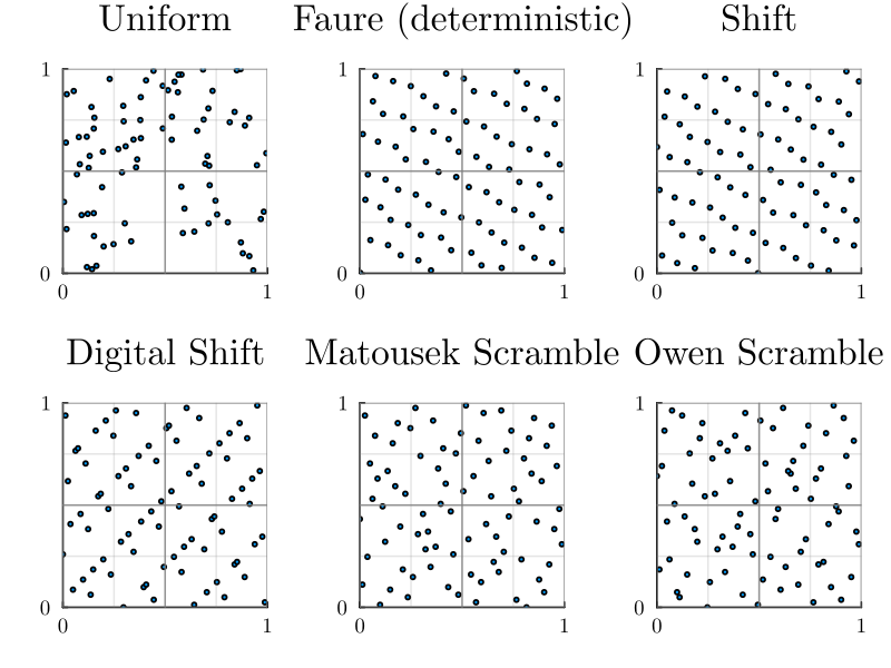
$(t,m,d)$-net visualization
Faure nets and their scrambled versions are digital $(t,m,d)$-net, which means they have strong equipartition properties. On the following plot, we can (visually) verify that with Nested Uniform Scrambling, it also works with Linear Matrix Scrambling and Digital Shift. You must see one point per rectangle of volume $1/b^m$. Points on the "left" border of rectangles are included, while those on the "right" are excluded. See Chapter 15.7 and Figure 15.10 for more details.
d1 = 1
d2 = 3 # you can try every combination of dimension (d1, d2)
x = x_nus # Owen Scramble, you can try x_lms and x_digital_shift
p = [plot(thickness_scaling = 1.5, aspect_ratio = :equal) for i in 0:m]
for i in 0:m
    j = m - i
    xᵢ = range(0, 1, step = 1 / b^(i))
    xⱼ = range(0, 1, step = 1 / b^(j))
    scatter!(p[i + 1], x[d1, :], x[d2, :], ms = 1.5, c = 1, grid = false)
    xlims!(p[i + 1], (0, 1.01))
    ylims!(p[i + 1], (0, 1.01))
    yticks!(p[i + 1], [0, 1])
    xticks!(p[i + 1], [0, 1])
    hline!(p[i + 1], xᵢ, c = :gray, alpha = 0.2)
    vline!(p[i + 1], xⱼ, c = :gray, alpha = 0.2)
end
plot(p..., size = (800, 600))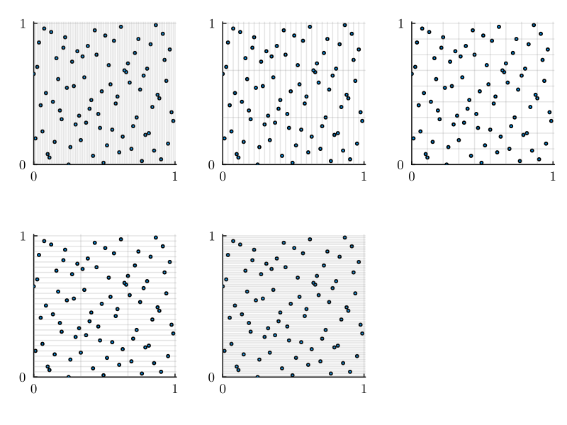
The package test suite uses the istmsnet helper to check whether a point set is a $(t,m,d)$-net. See the test suite for the exact checks when contributing a new sequence. It uses the excellent IntervalArithmetic.jl package.