Controlling Stochastic Differential Equations

In this tutorial, we show how to use SciMLSensitivity to control the time evolution of a system described by a stochastic differential equation (SDE). Specifically, we consider a continuously monitored qubit described by an SDE in the Ito sense with multiplicative scalar noise (see [1] for a reference):

\[dψ = b(ψ(t), Ω(t))ψ(t) dt + σ(ψ(t))ψ(t) dW_t .\]

We use a predictive model to map the quantum state of the qubit, ψ(t), at each time to the control parameter Ω(t) which rotates the quantum state about the x-axis of the Bloch sphere to ultimately prepare and stabilize the qubit in the excited state.

Copy-Pasteable Code

Before getting to the explanation, here's some code to start with. We will follow a full explanation of the definition and training process:

# load packages
using SciMLSensitivity, Optimization, OptimizationOptimisers
using StochasticDiffEq, DiffEqCallbacks, DiffEqNoiseProcess
using Zygote, Statistics, LinearAlgebra, Random
using Lux, Random, ComponentArrays
using Plots

rng = Random.default_rng()

#################################################
lr = 0.01f0
epochs = 100

numtraj = 16 # number of trajectories in parallel simulations for training
numtrajplot = 32 # .. for plotting

# time range for the solver
dt = 0.0005f0
tinterval = 0.05f0
tstart = 0.0f0
Nintervals = 20 # total number of intervals, total time = t_interval*Nintervals
tspan = (tstart, tinterval * Nintervals)
ts = Array(tstart:dt:(Nintervals * tinterval + dt)) # time array for noise grid

# Hamiltonian parameters
Δ = 20.0f0
Ωmax = 10.0f0 # control parameter (maximum amplitude)
κ = 0.3f0

# loss hyperparameters
C1 = Float32(1.0)  # evolution state fidelity

struct Parameters{flType, intType, tType}
    lr::flType
    epochs::intType
    numtraj::intType
    numtrajplot::intType
    dt::flType
    tinterval::flType
    tspan::tType
    Nintervals::intType
    ts::Vector{flType}
    Δ::flType
    Ωmax::flType
    κ::flType
    C1::flType
end

myparameters = Parameters{typeof(dt), typeof(numtraj), typeof(tspan)}(lr, epochs, numtraj,
    numtrajplot, dt,
    tinterval, tspan,
    Nintervals, ts,
    Δ, Ωmax, κ, C1)

################################################
# Define Neural Network

# state-aware
nn = Lux.Chain(Lux.Dense(4, 32, relu),
    Lux.Dense(32, 1, tanh))

p_nn, st = Lux.setup(rng, nn)
p_nn = ComponentArray(p_nn)

###############################################
# initial state anywhere on the Bloch sphere
function prepare_initial(dt, n_par)
    # shape 4 x n_par
    # input number of parallel realizations and dt for type inference
    # random position on the Bloch sphere
    theta = acos.(2 * rand(typeof(dt), n_par) .- 1)  # uniform sampling for cos(theta) between -1 and 1
    phi = rand(typeof(dt), n_par) * 2 * pi  # uniform sampling for phi between 0 and 2pi
    # real and imaginary parts ceR, cdR, ceI, cdI
    u0 = [
        cos.(theta / 2),
        sin.(theta / 2) .* cos.(phi),
        false * theta,
        sin.(theta / 2) .* sin.(phi)
    ]
    return vcat(transpose.(u0)...) # build matrix
end

# target state
# ψtar = |up>

u0 = prepare_initial(myparameters.dt, myparameters.numtraj)

###############################################
# Define SDE

function qubit_drift!(du, u, p, t)
    # expansion coefficients |Ψ> = ce |e> + cd |d>
    ceR, cdR, ceI, cdI = u # real and imaginary parts

    # Δ: atomic frequency
    # Ω: Rabi frequency for field in x direction
    # κ: spontaneous emission
    Δ, Ωmax, κ = p.myparameters
    nn_weights = p.p_nn
    Ω = (nn(u, nn_weights, st)[1] .* Ωmax)[1]

    @inbounds begin
        du[1] = 1 // 2 * (ceI * Δ - ceR * κ + cdI * Ω)
        du[2] = -cdI * Δ / 2 + 1 * ceR * (cdI * ceI + cdR * ceR) * κ + ceI * Ω / 2
        du[3] = 1 // 2 * (-ceR * Δ - ceI * κ - cdR * Ω)
        du[4] = cdR * Δ / 2 + 1 * ceI * (cdI * ceI + cdR * ceR) * κ - ceR * Ω / 2
    end
    return nothing
end

function qubit_diffusion!(du, u, p, t)
    ceR, cdR, ceI, cdI = u # real and imaginary parts

    κ = p.myparameters[end]

    du .= false

    @inbounds begin
        #du[1] = zero(ceR)
        du[2] += sqrt(κ) * ceR
        #du[3] = zero(ceR)
        du[4] += sqrt(κ) * ceI
    end
    return nothing
end

# normalization callback
condition(u, t, integrator) = true
function affect!(integrator)
    integrator.u .= integrator.u / norm(integrator.u)
end
callback = DiscreteCallback(condition, affect!, save_positions = (false, false))

CreateGrid(t, W1) = NoiseGrid(t, W1)
Zygote.@nograd CreateGrid #avoid taking grads of this function

# set scalar random process
W = sqrt(myparameters.dt) * randn(typeof(myparameters.dt), size(myparameters.ts)) #for 1 trajectory
W1 = cumsum([zero(myparameters.dt); W[1:(end - 1)]], dims = 1)
NG = CreateGrid(myparameters.ts, W1)

# get control pulses
p_all = ComponentArray(p_nn = p_nn,
    myparameters = [myparameters.Δ, myparameters.Ωmax, myparameters.κ])
# define SDE problem
prob = SDEProblem{true}(qubit_drift!, qubit_diffusion!, vec(u0[:, 1]), myparameters.tspan,
    p_all,
    callback = callback, noise = NG)

#########################################
# compute loss
function g(u, p, t)
    ceR = @view u[1, :, :]
    cdR = @view u[2, :, :]
    ceI = @view u[3, :, :]
    cdI = @view u[4, :, :]
    p[1] * mean((cdR .^ 2 + cdI .^ 2) ./ (ceR .^ 2 + cdR .^ 2 + ceI .^ 2 + cdI .^ 2))
end

function loss(p_nn; alg = EM(), sensealg = BacksolveAdjoint(autojacvec = ReverseDiffVJP()))
    pars = ComponentArray(p_nn = p_nn,
        myparameters = [myparameters.Δ, myparameters.Ωmax, myparameters.κ])
    u0 = prepare_initial(myparameters.dt, myparameters.numtraj)

    function prob_func(prob, i, repeat)
        # prepare initial state and applied control pulse
        u0tmp = deepcopy(vec(u0[:, i]))
        W = sqrt(myparameters.dt) * randn(typeof(myparameters.dt), size(myparameters.ts)) #for 1 trajectory
        W1 = cumsum([zero(myparameters.dt); W[1:(end - 1)]], dims = 1)
        NG = CreateGrid(myparameters.ts, W1)
        remake(prob,
            u0 = u0tmp,
            callback = callback,
            noise = NG)
    end
    _prob = remake(prob, p = pars)

    ensembleprob = EnsembleProblem(_prob,
        prob_func = prob_func,
        safetycopy = true)

    _sol = solve(ensembleprob, alg, EnsembleSerial(),
        sensealg = sensealg,
        saveat = myparameters.tinterval,
        dt = myparameters.dt,
        adaptive = false,
        trajectories = myparameters.numtraj, batch_size = myparameters.numtraj)
    A = convert(Array, _sol)

    l = g(A, [myparameters.C1], nothing)
    # returns loss value
    return l
end

#########################################
# visualization -- run for new batch
function visualize(p_nn; alg = EM())
    u0 = prepare_initial(myparameters.dt, myparameters.numtrajplot)
    pars = ComponentArray(p_nn = p_nn,
        myparameters = [myparameters.Δ, myparameters.Ωmax, myparameters.κ])

    function prob_func(prob, i, repeat)
        # prepare initial state and applied control pulse
        u0tmp = deepcopy(vec(u0[:, i]))
        W = sqrt(myparameters.dt) * randn(typeof(myparameters.dt), size(myparameters.ts)) #for 1 trajectory
        W1 = cumsum([zero(myparameters.dt); W[1:(end - 1)]], dims = 1)
        NG = CreateGrid(myparameters.ts, W1)

        remake(prob,
            p = pars,
            u0 = u0tmp,
            callback = callback,
            noise = NG)
    end

    ensembleprob = EnsembleProblem(prob,
        prob_func = prob_func,
        safetycopy = true)

    u = solve(ensembleprob, alg, EnsembleThreads(),
        saveat = myparameters.tinterval,
        dt = myparameters.dt,
        adaptive = false, #abstol=1e-6, reltol=1e-6,
        trajectories = myparameters.numtrajplot,
        batch_size = myparameters.numtrajplot)

    ceR = @view u[1, :, :]
    cdR = @view u[2, :, :]
    ceI = @view u[3, :, :]
    cdI = @view u[4, :, :]
    infidelity = @. (cdR^2 + cdI^2) / (ceR^2 + cdR^2 + ceI^2 + cdI^2)
    meaninfidelity = mean(infidelity)
    loss = myparameters.C1 * meaninfidelity

    @info "Loss: " loss

    fidelity = @. (ceR^2 + ceI^2) / (ceR^2 + cdR^2 + ceI^2 + cdI^2)

    mf = mean(fidelity, dims = 2)[:]
    sf = std(fidelity, dims = 2)[:]

    pl1 = plot(0:(myparameters.Nintervals), mf,
        ribbon = sf,
        ylim = (0, 1), xlim = (0, myparameters.Nintervals),
        c = 1, lw = 1.5, xlabel = "steps i", ylabel = "Fidelity", legend = false)

    pl = plot(pl1, legend = false, size = (400, 360))
    return pl, loss
end

# burn-in loss
l = loss(p_nn)
# callback to visualize training
visualization_callback = function (state, l; doplot = false)
    println(l)

    if doplot
        pl, _ = visualize(state.u)
        display(pl)
    end

    return false
end

# Display the ODE with the initial parameter values.
visualization_callback((; u = p_nn), l; doplot = true)

###################################
# training loop
@info "Start Training.."

# optimize the parameters for a few epochs with Adam on time span
# Setup and run the optimization
adtype = Optimization.AutoForwardDiff()
optf = Optimization.OptimizationFunction((x, p) -> loss(x), adtype)

optprob = Optimization.OptimizationProblem(optf, p_nn)
res = Optimization.solve(optprob, OptimizationOptimisers.Adam(myparameters.lr),
    callback = visualization_callback,
    maxiters = 100)

# plot optimized control
visualization_callback(res, loss(res.u); doplot = true)

false

Step-by-step description

Load packages

using SciMLSensitivity
using Optimization, OptimizationOptimisers, Zygote
using StochasticDiffEq, DiffEqCallbacks, DiffEqNoiseProcess
using Statistics, LinearAlgebra
using Lux, Random, ComponentArrays
using Plots

Parameters

We define the parameters of the qubit and hyperparameters of the training process.

lr = 0.01f0
epochs = 100

numtraj = 16 # number of trajectories in parallel simulations for training
numtrajplot = 32 # .. for plotting

rng = Random.default_rng()

# time range for the solver
dt = 0.0005f0
tinterval = 0.05f0
tstart = 0.0f0
Nintervals = 20 # total number of intervals, total time = t_interval*Nintervals
tspan = (tstart, tinterval * Nintervals)
ts = Array(tstart:dt:(Nintervals * tinterval + dt)) # time array for noise grid

# Hamiltonian parameters
Δ = 20.0f0
Ωmax = 10.0f0 # control parameter (maximum amplitude)
κ = 0.3f0

# loss hyperparameters
C1 = Float32(1.0)  # evolution state fidelity

struct Parameters{flType, intType, tType}
    lr::flType
    epochs::intType
    numtraj::intType
    numtrajplot::intType
    dt::flType
    tinterval::flType
    tspan::tType
    Nintervals::intType
    ts::Vector{flType}
    Δ::flType
    Ωmax::flType
    κ::flType
    C1::flType
end

myparameters = Parameters{typeof(dt), typeof(numtraj), typeof(tspan)}(lr, epochs, numtraj,
    numtrajplot, dt,
    tinterval, tspan,
    Nintervals, ts,
    Δ, Ωmax, κ, C1)

Main.Parameters{Float32, Int64, Tuple{Float32, Float32}}(0.01f0, 100, 16, 32, 0.0005f0, 0.05f0, (0.0f0, 1.0f0), 20, Float32[0.0, 0.0005, 0.001, 0.0015, 0.002, 0.0025, 0.003, 0.0035, 0.004, 0.0045  …  0.996, 0.9965, 0.997, 0.9975, 0.998, 0.9985, 0.999, 0.9995, 1.0, 1.0005], 20.0f0, 10.0f0, 0.3f0, 1.0f0)

In plain terms, the quantities that were defined are:

• lr = learning rate of the optimizer
• epochs = number of epochs in the training process
• numtraj = number of simulated trajectories in the training process
• numtrajplot = number of simulated trajectories to visualize the performance
• dt = time step for solver (initial dt if adaptive)
• tinterval = time spacing between checkpoints
• tspan = time span
• Nintervals = number of checkpoints
• ts = discretization of the entire time interval, used for NoiseGrid
• Δ = detuning between the qubit and the laser
• Ωmax = maximum frequency of the control laser
• κ = decay rate
• C1 = loss function hyperparameter

Controller

We use a neural network to control the parameter Ω(t). Alternatively, one could also, e.g., use polynomials, interpolations, etc. but we use a neural network to demonstrate coolness factor and complexity.

# state-aware
nn = Lux.Chain(Lux.Dense(4, 32, relu),
    Lux.Dense(32, 1, tanh))

p_nn, st = Lux.setup(rng, nn)
p_nn = ComponentArray(p_nn)

ComponentVector{Float32}(layer_1 = (weight = Float32[1.4524051 0.79613537 -0.32291588 0.5087743; 0.41646546 0.19238596 -0.40128696 1.0920839; … ; -1.4312388 -1.6194137 1.5212426 -1.3256183; -1.3630639 0.15811911 1.5048242 -0.39531958], bias = Float32[0.08788425, 0.30204558, 0.026035547, -0.41491646, 0.3916874, 0.12014347, -0.3181302, 0.40205657, 0.39288568, -0.35784853  …  -0.16605216, -0.39021218, -0.103458285, -0.09773654, -0.47864175, -0.12336129, -0.16305667, -0.49864048, 0.22408223, -0.4181705]), layer_2 = (weight = Float32[0.37897933 -0.39741853 … -0.06963005 -0.41279912], bias = Float32[-0.15967411]))

Initial state

We prepare n_par initial states, uniformly distributed over the Bloch sphere. To avoid complex numbers in our simulations, we split the state of the qubit

\[ ψ(t) = c_e(t) (1,0) + c_d(t) (0,1)\]

into its real and imaginary part.

# initial state anywhere on the Bloch sphere
function prepare_initial(dt, n_par)
    # shape 4 x n_par
    # input number of parallel realizations and dt for type inference
    # random position on the Bloch sphere
    theta = acos.(2 * rand(typeof(dt), n_par) .- 1)  # uniform sampling for cos(theta) between -1 and 1
    phi = rand(typeof(dt), n_par) * 2 * pi  # uniform sampling for phi between 0 and 2pi
    # real and imaginary parts ceR, cdR, ceI, cdI
    u0 = [
        cos.(theta / 2),
        sin.(theta / 2) .* cos.(phi),
        false * theta,
        sin.(theta / 2) .* sin.(phi)
    ]
    return vcat(transpose.(u0)...) # build matrix
end

# target state
# ψtar = |e>

u0 = prepare_initial(myparameters.dt, myparameters.numtraj)

4×16 Matrix{Float32}:
  0.948068   0.958473  0.768489  0.799253  …   0.726856  0.70266   0.949439
  0.124237  -0.188683  0.559156  0.176302      0.505944  0.311865  0.301735
  0.0        0.0       0.0       0.0           0.0       0.0       0.0
 -0.2928    -0.213842  0.311078  0.574553     -0.464436  0.639539  0.0867228

Defining the SDE

We define the drift and diffusion term of the qubit. The SDE doesn't preserve the norm of the quantum state. To ensure the normalization of the state, we add a DiscreteCallback after each time step. Further, we use a NoiseGrid from the DiffEqNoiseProcess package, as one possibility to simulate a 1D Brownian motion. Note that the NN is placed directly into the drift function, thus the control parameter Ω is continuously updated.

# Define SDE
function qubit_drift!(du, u, p, t)
    # expansion coefficients |Ψ> = ce |e> + cd |d>
    ceR, cdR, ceI, cdI = u # real and imaginary parts

    # Δ: atomic frequency
    # Ω: Rabi frequency for field in x direction
    # κ: spontaneous emission
    Δ, Ωmax, κ = p.myparameters
    nn_weights = p.p_nn
    Ω = (nn(u, nn_weights, st)[1] .* Ωmax)[1]

    @inbounds begin
        du[1] = 1 // 2 * (ceI * Δ - ceR * κ + cdI * Ω)
        du[2] = -cdI * Δ / 2 + 1 * ceR * (cdI * ceI + cdR * ceR) * κ + ceI * Ω / 2
        du[3] = 1 // 2 * (-ceR * Δ - ceI * κ - cdR * Ω)
        du[4] = cdR * Δ / 2 + 1 * ceI * (cdI * ceI + cdR * ceR) * κ - ceR * Ω / 2
    end
    return nothing
end

function qubit_diffusion!(du, u, p, t)
    ceR, cdR, ceI, cdI = u # real and imaginary parts

    κ = p[end]

    du .= false

    @inbounds begin
        #du[1] = zero(ceR)
        du[2] += sqrt(κ) * ceR
        #du[3] = zero(ceR)
        du[4] += sqrt(κ) * ceI
    end
    return nothing
end

# normalization callback
condition(u, t, integrator) = true
function affect!(integrator)
    integrator.u .= integrator.u / norm(integrator.u)
end
callback = DiscreteCallback(condition, affect!, save_positions = (false, false))

CreateGrid(t, W1) = NoiseGrid(t, W1)
Zygote.@nograd CreateGrid #avoid taking grads of this function

# set scalar random process
W = sqrt(myparameters.dt) * randn(typeof(myparameters.dt), size(myparameters.ts)) #for 1 trajectory
W1 = cumsum([zero(myparameters.dt); W[1:(end - 1)]], dims = 1)
NG = CreateGrid(myparameters.ts, W1)

# get control pulses
p_all = ComponentArray(p_nn = p_nn,
    myparameters = [myparameters.Δ; myparameters.Ωmax; myparameters.κ])
# define SDE problem
prob = SDEProblem{true}(qubit_drift!, qubit_diffusion!, vec(u0[:, 1]), myparameters.tspan,
    p_all,
    callback = callback, noise = NG)

SDEProblem with uType Vector{Float32} and tType Float32. In-place: true
Non-trivial mass matrix: false
timespan: (0.0f0, 1.0f0)
u0: 4-element Vector{Float32}:
  0.9480682
  0.12423742
  0.0
 -0.2927998

Compute loss function

We'd like to prepare the excited state of the qubit. An appropriate choice for the loss function is the infidelity of the state ψ(t) with respect to the excited state. We create a parallelized EnsembleProblem, where the prob_func creates a new NoiseGrid for every trajectory and loops over the initial states. The number of parallel trajectories and the used batch size can be tuned by the kwargs trajectories=.. and batchsize=.. in the solve call. See also the parallel ensemble simulation docs for a description of the available ensemble algorithms. To optimize only the parameters of the neural network, we use pars = [p; myparameters.Δ; myparameters.Ωmax; myparameters.κ]

# compute loss
function g(u, p, t)
    ceR = @view u[1, :, :]
    cdR = @view u[2, :, :]
    ceI = @view u[3, :, :]
    cdI = @view u[4, :, :]
    p[1] * mean((cdR .^ 2 + cdI .^ 2) ./ (ceR .^ 2 + cdR .^ 2 + ceI .^ 2 + cdI .^ 2))
end

function loss(p_nn; alg = EM(), sensealg = BacksolveAdjoint(autojacvec = ReverseDiffVJP()))
    pars = ComponentArray(p_nn = p_nn,
        myparameters = [myparameters.Δ, myparameters.Ωmax,
            myparameters.κ])
    u0 = prepare_initial(myparameters.dt, myparameters.numtraj)

    function prob_func(prob, i, repeat)
        # prepare initial state and applied control pulse
        u0tmp = deepcopy(vec(u0[:, i]))
        W = sqrt(myparameters.dt) * randn(typeof(myparameters.dt), size(myparameters.ts)) #for 1 trajectory
        W1 = cumsum([zero(myparameters.dt); W[1:(end - 1)]], dims = 1)
        NG = CreateGrid(myparameters.ts, W1)

        remake(prob,
            p = pars,
            u0 = u0tmp,
            callback = callback,
            noise = NG)
    end

    ensembleprob = EnsembleProblem(prob,
        prob_func = prob_func,
        safetycopy = true)

    _sol = solve(ensembleprob, alg, EnsembleThreads(),
        sensealg = sensealg,
        saveat = myparameters.tinterval,
        dt = myparameters.dt,
        adaptive = false,
        trajectories = myparameters.numtraj, batch_size = myparameters.numtraj)
    A = convert(Array, _sol)

    l = g(A, [myparameters.C1], nothing)
    # returns loss value
    return l
end

loss (generic function with 1 method)

Visualization

To visualize the performance of the controller, we plot the mean value and standard deviation of the fidelity of a bunch of trajectories (myparameters.numtrajplot) as a function of the time steps at which loss values are computed.

function visualize(p_nn; alg = EM())
    u0 = prepare_initial(myparameters.dt, myparameters.numtrajplot)
    pars = ComponentArray(p_nn = p_nn,
        myparameters = [myparameters.Δ, myparameters.Ωmax,
            myparameters.κ])

    function prob_func(prob, i, repeat)
        # prepare initial state and applied control pulse
        u0tmp = deepcopy(vec(u0[:, i]))
        W = sqrt(myparameters.dt) * randn(typeof(myparameters.dt), size(myparameters.ts)) #for 1 trajectory
        W1 = cumsum([zero(myparameters.dt); W[1:(end - 1)]], dims = 1)
        NG = CreateGrid(myparameters.ts, W1)

        remake(prob,
            p = pars,
            u0 = u0tmp,
            callback = callback,
            noise = NG)
    end

    ensembleprob = EnsembleProblem(prob,
        prob_func = prob_func,
        safetycopy = true)

    u = solve(ensembleprob, alg, EnsembleThreads(),
        saveat = myparameters.tinterval,
        dt = myparameters.dt,
        adaptive = false, #abstol=1e-6, reltol=1e-6,
        trajectories = myparameters.numtrajplot,
        batch_size = myparameters.numtrajplot)

    ceR = @view u[1, :, :]
    cdR = @view u[2, :, :]
    ceI = @view u[3, :, :]
    cdI = @view u[4, :, :]
    infidelity = @. (cdR^2 + cdI^2) / (ceR^2 + cdR^2 + ceI^2 + cdI^2)
    meaninfidelity = mean(infidelity)
    loss = myparameters.C1 * meaninfidelity

    @info "Loss: " loss

    fidelity = @. (ceR^2 + ceI^2) / (ceR^2 + cdR^2 + ceI^2 + cdI^2)

    mf = mean(fidelity, dims = 2)[:]
    sf = std(fidelity, dims = 2)[:]

    pl1 = plot(0:(myparameters.Nintervals), mf,
        ribbon = sf,
        ylim = (0, 1), xlim = (0, myparameters.Nintervals),
        c = 1, lw = 1.5, xlabel = "steps i", ylabel = "Fidelity", legend = false)

    pl = plot(pl1, legend = false, size = (400, 360))
    return pl, loss
end
# callback to visualize training
visualization_callback = function (state, l; doplot = false)
    println(l)

    if doplot
        pl, _ = visualize(state.u)
        display(pl)
    end

    return false
end

#7 (generic function with 1 method)

Training

We use the Adam optimizer to optimize the parameters of the neural network. In each epoch, we draw new initial quantum states, compute the forward evolution, and, subsequently, the gradients of the loss function with respect to the parameters of the neural network. sensealg allows one to switch between the different sensitivity modes. InterpolatingAdjoint and BacksolveAdjoint are the two possible continuous adjoint sensitivity methods. The necessary correction between Ito and Stratonovich integrals is computed under the hood in the SciMLSensitivity package.

# optimize the parameters for a few epochs with Adam on time span
# Setup and run the optimization
adtype = Optimization.AutoForwardDiff()
optf = Optimization.OptimizationFunction((x, p) -> loss(x), adtype)

optprob = Optimization.OptimizationProblem(optf, p_nn)
res = Optimization.solve(optprob, OptimizationOptimisers.Adam(myparameters.lr),
    callback = visualization_callback,
    maxiters = 100)

# plot optimized control
visualization_callback(res, loss(res.u); doplot = true)

false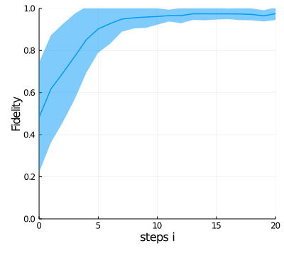

References

[1] Schäfer, Frank, Pavel Sekatski, Martin Koppenhöfer, Christoph Bruder, and Michal Kloc. "Control of stochastic quantum dynamics by differentiable programming." Machine Learning: Science and Technology 2, no. 3 (2021): 035004.