Training Neural Networks in Hybrid Differential Equations

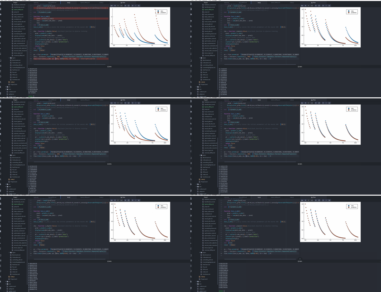
Hybrid differential equations are differential equations with implicit or explicit discontinuities as specified by callbacks. In the following example, explicit dosing times are given for a pharmacometric model and the universal differential equation is trained to uncover the missing dynamical equations.

using ComponentArrays, Random, SciMLSensitivity,
      Lux, OrdinaryDiffEq, Plots, Optimization, OptimizationOptimisers, DiffEqCallbacks

u0 = Float32[2.0; 0.0]
datasize = 100
tspan = (0.0f0, 10.5f0)
dosetimes = [1.0, 2.0, 4.0, 8.0]

function affect!(integrator)
    integrator.u = integrator.u .+ 1
end
cb_ = PresetTimeCallback(dosetimes, affect!, save_positions = (false, false))
function trueODEfunc(du, u, p, t)
    du .= -u
end
t = range(tspan[1], tspan[2], length = datasize)

prob = ODEProblem(trueODEfunc, u0, tspan)
ode_data = Array(solve(prob, Tsit5(), callback = cb_, saveat = t))

dudt2 = Lux.Chain(Lux.Dense(2, 50, tanh), Lux.Dense(50, 2))
ps, st = Lux.setup(Random.default_rng(), dudt2)

function dudt(du, u, p, t)
    du[1:2] .= -u[1:2]
    du[3:end] .= first(dudt2(u[1:2], p, st))
end
z0 = Float32[u0; u0]
prob = ODEProblem(dudt, z0, tspan)

affect!(integrator) = integrator.u[1:2] .= integrator.u[3:end]
cb = PresetTimeCallback(dosetimes, affect!, save_positions = (false, false))

function predict_n_ode(p)
    _prob = remake(prob, p = p)
    Array(solve(_prob, Tsit5(), u0 = z0, p = p, callback = cb, saveat = t,
        sensealg = ReverseDiffAdjoint()))[1:2, :]
    #Array(solve(prob,Tsit5(),u0=z0,p=p,saveat=t))[1:2,:]
end

function loss_n_ode(p, _)
    pred = predict_n_ode(p)
    loss = sum(abs2, ode_data .- pred)
    loss
end
loss_n_ode(ps, nothing)

cba = function (state, l; doplot = false) #callback function to observe training
    pred = predict_n_ode(state.u)
    display(sum(abs2, ode_data .- pred))
    # plot current prediction against data
    pl = scatter(t, ode_data[1, :], label = "data")
    scatter!(pl, t, pred[1, :], label = "prediction")
    display(plot(pl))
    return false
end

res = solve(
    OptimizationProblem(OptimizationFunction(loss_n_ode, AutoZygote()),
        ComponentArray(ps)),
    OptimizationOptimisers.Adam(0.05); callback = cba, maxiters = 1000)

retcode: Default
u: ComponentVector{Float32}(layer_1 = (weight = Float32[0.59040236 0.8391867; -1.6001942 1.843297; … ; 1.0588355 -0.22815108; 0.4023668 -1.6167738], bias = Float32[-0.10889249, 0.66669416, 0.28391287, 0.102803975, -0.30080023, -0.42324457, 0.22944008, 0.40388966, 0.56512636, -0.13230795  …  0.42912126, 0.22216171, -0.2691199, 0.57730913, 0.84370315, 0.3410861, -1.0224549, 0.05398032, -0.13240246, -0.6898274]), layer_2 = (weight = Float32[0.109119736 -0.0014516157 … 0.08404693 -0.13104993; 0.053615402 0.021942448 … 0.24956617 -0.15190288], bias = Float32[-0.38148847, -0.007898975]))

Note on Sensitivity Methods

The continuous adjoint sensitivities BacksolveAdjoint, InterpolatingAdjoint, and QuadratureAdjoint are compatible with events for ODEs. BacksolveAdjoint and InterpolatingAdjoint can also handle events for SDEs. Use BacksolveAdjoint if the event terminates the time evolution and several states are saved. Currently, the continuous adjoint sensitivities do not support multiple events per time point.

All methods based on discrete sensitivity analysis via automatic differentiation, like ReverseDiffAdjoint, TrackerAdjoint, or ForwardDiffSensitivity are the methods to use (and ReverseDiffAdjoint is demonstrated above), are compatible with events. This applies to SDEs, DAEs, and DDEs as well.