Optimization of Ordinary Differential Equations
Copy-Paste Code
If you want to just get things running, try the following! Explanation will follow.
using DifferentialEquations, Optimization, OptimizationPolyalgorithms, OptimizationOptimJL,
      SciMLSensitivity, Zygote, Plots

function lotka_volterra!(du, u, p, t)
  x, y = u
  α, β, δ, γ = p
  du[1] = dx = α*x - β*x*y
  du[2] = dy = -δ*y + γ*x*y
end

# Initial condition
u0 = [1.0, 1.0]

# Simulation interval and intermediary points
tspan = (0.0, 10.0)
tsteps = 0.0:0.1:10.0

# LV equation parameter. p = [α, β, δ, γ]
p = [1.5, 1.0, 3.0, 1.0]

# Setup the ODE problem, then solve
prob = ODEProblem(lotka_volterra!, u0, tspan, p)
sol = solve(prob, Tsit5())

# Plot the solution
using Plots
plot(sol)
savefig("LV_ode.png")

function loss(p)
  sol = solve(prob, Tsit5(), p=p, saveat = tsteps)
  loss = sum(abs2, sol.-1)
  return loss, sol
end

callback = function (p, l, pred)
  display(l)
  plt = plot(pred, ylim = (0, 6))
  display(plt)
  # Tell Optimization.solve to not halt the optimization. If return true, then
  # optimization stops.
  return false
end

adtype = Optimization.AutoZygote()
optf = Optimization.OptimizationFunction((x,p)->loss(x), adtype)
optprob = Optimization.OptimizationProblem(optf, p)

result_ode = Optimization.solve(optprob, PolyOpt(),
                                callback = callback,
                                maxiters = 100)
u: 4-element Vector{Float64}:
1.526796365699704
1.5268447127347722
2.038104450096957
2.0380008543235464Explanation
First let's create a Lotka-Volterra ODE using DifferentialEquations.jl. For more details, see the DifferentialEquations.jl documentation. The Lotka-Volterra equations have the form:
\[\begin{aligned} \frac{dx}{dt} &= \alpha x - \beta x y \\ \frac{dy}{dt} &= -\delta y + \gamma x y \\ \end{aligned}\]
using DifferentialEquations, Optimization, OptimizationPolyalgorithms, OptimizationOptimJL,
      SciMLSensitivity, Zygote, Plots

function lotka_volterra!(du, u, p, t)
  x, y = u
  α, β, δ, γ = p
  du[1] = dx = α*x - β*x*y
  du[2] = dy = -δ*y + γ*x*y
end

# Initial condition
u0 = [1.0, 1.0]

# Simulation interval and intermediary points
tspan = (0.0, 10.0)
tsteps = 0.0:0.1:10.0

# LV equation parameter. p = [α, β, δ, γ]
p = [1.5, 1.0, 3.0, 1.0]

# Setup the ODE problem, then solve
prob = ODEProblem(lotka_volterra!, u0, tspan, p)
sol = solve(prob, Tsit5())

# Plot the solution
using Plots
plot(sol)
savefig("LV_ode.png")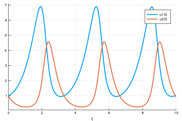
For this first example, we do not yet include a neural network. We take AD-compatible solve function function that takes the parameters and an initial condition and returns the solution of the differential equation. Next we choose a loss function. Our goal will be to find parameters that make the Lotka-Volterra solution constant x(t)=1, so we define our loss as the squared distance from 1.
function loss(p)
  sol = solve(prob, Tsit5(), p=p, saveat = tsteps)
  loss = sum(abs2, sol.-1)
  return loss, sol
end
loss (generic function with 1 method)Lastly, we use the Optimization.solve function to train the parameters using ADAM to arrive at parameters which optimize for our goal. Optimization.solve allows defining a callback that will be called at each step of our training loop. It takes in the current parameter vector and the returns of the last call to the loss function. We will display the current loss and make a plot of the current situation:
callback = function (p, l, pred)
  display(l)
  plt = plot(pred, ylim = (0, 6))
  display(plt)
  # Tell Optimization.solve to not halt the optimization. If return true, then
  # optimization stops.
  return false
end
#1 (generic function with 1 method)Let's optimize the model.
adtype = Optimization.AutoZygote()
optf = Optimization.OptimizationFunction((x,p)->loss(x), adtype)
optprob = Optimization.OptimizationProblem(optf, p)

result_ode = Optimization.solve(optprob, PolyOpt(),
                                callback = callback,
                                maxiters = 100)
u: 4-element Vector{Float64}:
1.526796365699704
1.5268447127347722
2.038104450096957
2.0380008543235464In just seconds we found parameters which give a relative loss of 1e-16! We can get the final loss with result_ode.minimum, and get the optimal parameters with result_ode.u. For example, we can plot the final outcome and show that we solved the control problem and successfully found parameters to make the ODE solution constant:
remade_solution = solve(remake(prob, p = result_ode.u), Tsit5(),
                        saveat = tsteps)
plot(remade_solution, ylim = (0, 6))