Event Handling and Callback Functions

DifferentialEquations.jl allows for using callback functions to inject user code into the solver algorithms. It allows for safely and accurately applying events and discontinuities. Multiple callbacks can be chained together, and these callback types can be used to build libraries of extension behavior.

The Callback Types

The callback types are defined as follows. There are three primitive callback types: the ContinuousCallback, DiscreteCallback and the VectorContinuousCallback:

• The ContinuousCallback is applied when a given continuous condition function hits zero. This hitting can happen even within an integration step, and the solver must be able to detect it and adjust the integration step accordingly. This type of callback implements what is known in other problem-solving environments as an Event.
• The DiscreteCallback is applied when its condition function is true, but the condition is only evaluated at the end of every integration step.
• The VectorContinuousCallback works like a vector of ContinuousCallbacks and lets the user specify a vector of continuous callbacks, each with simultaneous rootfinding equations. The effect that is applied is the effect corresponding to the first (earliest) condition that is satisfied. A VectorContinuousCallback is more efficient than a CallbackSet of ContinuousCallbacks as the number of callbacks grows. As such, it's a slightly more involved definition which gives better scaling.

ContinuousCallback

DiscreteCallback

CallbackSet

VectorContinuousCallback

Using Callbacks

The callback type is then sent to the solver (or the integrator) via the callback keyword argument:

sol = solve(prob, alg, callback = cb)

You can supply nothing, a single DiscreteCallback or ContinuousCallback or VectorContinuousCallback, or a CallbackSet.

Note About Saving

When a callback is supplied, the default saving behavior is turned off. This is because otherwise, events would “double save” one of the values. To re-enable the standard saving behavior, one must have the first save_positions value be true for at least one callback.

Modifying the Stepping Within A Callback

A common issue with callbacks is that they cause a large discontinuous change, and so it may be wise to pull down dt after such a change. To control the timestepping from a callback, please see the timestepping controls in the integrator interface. Specifically, set_proposed_dt! is used to set the next stepsize, and terminate! can be used to cause the simulation to stop.

DiscreteCallback Examples

Example 1: Interventions at Preset Times

Assume we have a patient whose internal drug concentration follows exponential decay, i.e. the linear ODE with a negative coefficient:

import DifferentialEquations as DE
import SciMLBase
import DiffEqCallbacks: PresetTimeCallback # no longer reexported by DifferentialEquations v8
function f(du, u, p, t)
    du[1] = -u[1]
    return
end
u0 = [10.0]
const V = 1
prob = DE.ODEProblem(f, u0, (0.0, 10.0))
sol = DE.solve(prob, DE.Tsit5())
import Plots: plot
plot(sol)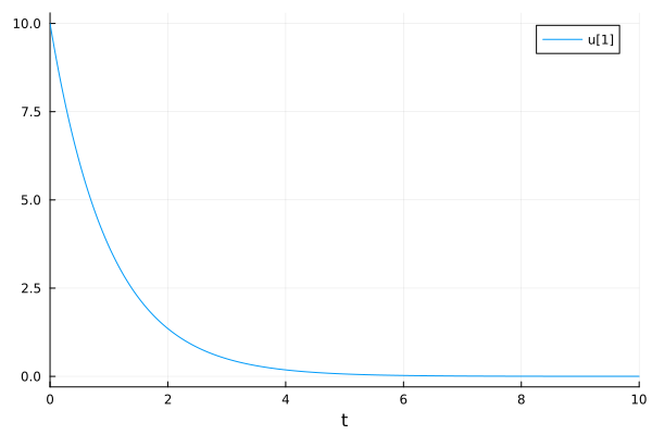

Now assume we wish to give the patient a dose of 10 at time t==4. For this, we can use a DiscreteCallback which will only be true at t==4:

condition(u, t, integrator) = t == 4
affect!(integrator) = integrator.u[1] += 10
cb = DE.DiscreteCallback(condition, affect!)

DiscreteCallback{typeof(Main.condition), typeof(Main.affect!), typeof(SciMLBase.INITIALIZE_DEFAULT), typeof(SciMLBase.FINALIZE_DEFAULT), Nothing, Tuple{}}(Main.condition, Main.affect!, SciMLBase.INITIALIZE_DEFAULT, SciMLBase.FINALIZE_DEFAULT, Bool[1, 1], nothing, (), true)

If we then solve with this callback enabled, we see no change:

sol = DE.solve(prob, DE.Tsit5(), callback = cb)
plot(sol)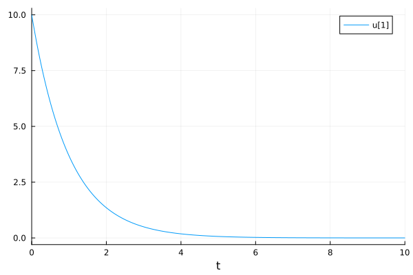

The reason there is no change is because the DiscreteCallback only applies at a specific time, and the integrator never hit that time. Thus we would like to force the ODE solver to step exactly at t=4 so that the condition can be applied. We can do that with the tstops argument:

sol = DE.solve(prob, DE.Tsit5(), callback = cb, tstops = [4.0])
plot(sol)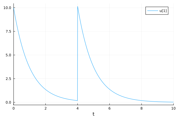

and thus we achieve the desired result.

Performing multiple doses then just requires that we have multiple points which are hit. For example, to dose at time t=4 and t=8, we can do the following:

dosetimes = [4.0, 8.0]
condition(u, t, integrator) = t ∈ dosetimes
affect!(integrator) = integrator.u[1] += 10
cb = DE.DiscreteCallback(condition, affect!)
sol = DE.solve(prob, DE.Tsit5(), callback = cb, tstops = dosetimes)
plot(sol)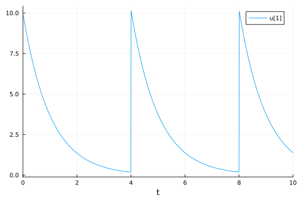

We can then use this mechanism to make the model arbitrarily complex. For example, let's say there's now 3 dose times, but the dose only triggers if the current concentration is below 1.0. Additionally, the dose is now 10t instead of just 10. This model is implemented as simply:

dosetimes = [4.0, 6.0, 8.0]
condition(u, t, integrator) = t ∈ dosetimes && (u[1] < 1.0)
affect!(integrator) = integrator.u[1] += 10 * integrator.t
cb = DE.DiscreteCallback(condition, affect!)
sol = DE.solve(prob, DE.Tsit5(), callback = cb, tstops = dosetimes)
plot(sol)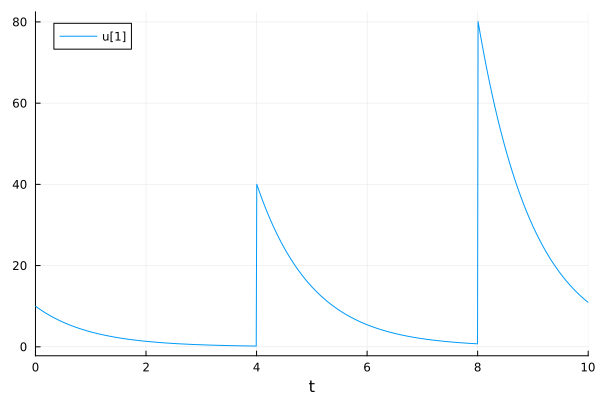

PresetTimeCallback

Because events at preset times is a very common occurrence, DifferentialEquations.jl provides a pre-built callback in the Callback Library. The PresetTimeCallback(tstops,affect!) takes an array of times and an affect! function to apply. Thus to do the simple 2 dose example with this callback, we could do the following:

dosetimes = [4.0, 8.0]
affect!(integrator) = integrator.u[1] += 10
cb = PresetTimeCallback(dosetimes, affect!)
sol = DE.solve(prob, DE.Tsit5(), callback = cb)
plot(sol)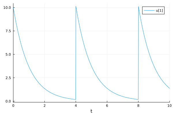

Notice that this version will automatically set the tstops for you.

Example 2: A Control Problem

Another example of a DiscreteCallback is a control problem switching parameters. Our parameterized ODE system is as follows:

Our ODE function will use this field as follows:

function f(du, u, p, t)
    du[1] = -0.5 * u[1] + p
    du[2] = -0.5 * u[2]
    return
end

f (generic function with 1 method)

Now we will setup our control mechanism. It will be a simple setup which uses set timepoints at which we will change p. At t=5.0 we will want to increase the value of p, and at t=8.0 we will want to decrease the value of p. Using the DiscreteCallback interface, we code these conditions as follows:

const tstop1 = [5.0]
const tstop2 = [8.0]

condition(u, t, integrator) = t in tstop1
condition2(u, t, integrator) = t in tstop2

condition2 (generic function with 1 method)

Now we have to apply an effect when these conditions are reached. When condition is hit (at t=5.0), we will increase p to 1.5. When condition2 is reached, we will decrease p to -1.5. This is done via the functions:

function affect!(integrator)
    integrator.p = 1.5
    return
end

function affect2!(integrator)
    integrator.p = -1.5
    return
end

affect2! (generic function with 1 method)

With these functions we can build our callbacks:

import DifferentialEquations as DE
save_positions = (true, true)

cb = DE.DiscreteCallback(condition, affect!; save_positions)

save_positions = (false, true)

cb2 = DE.DiscreteCallback(condition2, affect2!; save_positions)

cbs = DE.CallbackSet(cb, cb2)

CallbackSet{Tuple{}, Tuple{DiscreteCallback{typeof(Main.condition), typeof(Main.affect!), typeof(SciMLBase.INITIALIZE_DEFAULT), typeof(SciMLBase.FINALIZE_DEFAULT), Nothing, Tuple{}}, DiscreteCallback{typeof(Main.condition2), typeof(Main.affect2!), typeof(SciMLBase.INITIALIZE_DEFAULT), typeof(SciMLBase.FINALIZE_DEFAULT), Nothing, Tuple{}}}}((), (DiscreteCallback{typeof(Main.condition), typeof(Main.affect!), typeof(SciMLBase.INITIALIZE_DEFAULT), typeof(SciMLBase.FINALIZE_DEFAULT), Nothing, Tuple{}}(Main.condition, Main.affect!, SciMLBase.INITIALIZE_DEFAULT, SciMLBase.FINALIZE_DEFAULT, Bool[1, 1], nothing, (), true), DiscreteCallback{typeof(Main.condition2), typeof(Main.affect2!), typeof(SciMLBase.INITIALIZE_DEFAULT), typeof(SciMLBase.FINALIZE_DEFAULT), Nothing, Tuple{}}(Main.condition2, Main.affect2!, SciMLBase.INITIALIZE_DEFAULT, SciMLBase.FINALIZE_DEFAULT, Bool[0, 1], nothing, (), true)))

Now we define our initial condition. We will start at [10.0;10.0] with p=0.0.

u0 = [10.0; 10.0]
p = 0.0
prob = DE.ODEProblem(f, u0, (0.0, 10.0), p)

ODEProblem with uType Vector{Float64} and tType Float64. In-place: true
Non-trivial mass matrix: false
timespan: (0.0, 10.0)
u0: 2-element Vector{Float64}:
 10.0
 10.0

Lastly we solve the problem. Note that we must pass tstop values of 5.0 and 8.0 to ensure the solver hits those timepoints exactly:

const tstop = [5.0; 8.0]
sol = DE.solve(prob, DE.Tsit5(), callback = cbs, tstops = tstop)
import Plots: plot
plot(sol)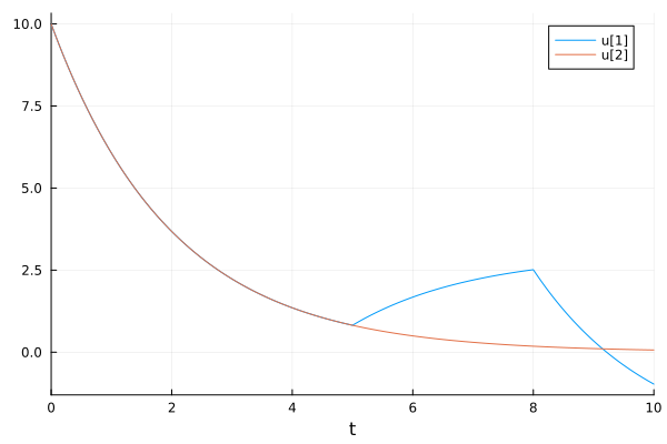

It's clear from the plot how the controls affected the outcome.

Example 3: AutoAbstol

MATLAB's Simulink has the option for an automatic absolute tolerance. In this example we will implement a callback which will add this behavior to any JuliaDiffEq solver which implements the integrator and callback interface.

The algorithm is as follows. The default value is set to start at 1e-6, though we will give the user an option for this choice. Then as the simulation progresses, at each step the absolute tolerance is set to the maximum value that has been reached so far times the relative tolerance. This is the behavior that we will implement in affect!.

Since the effect is supposed to occur every timestep, we use the trivial condition:

condition = function (u, t, integrator)
    return true
end

#2 (generic function with 1 method)

which always returns true. For our effect we will overload the call on a type. This type will have a value for the current maximum. By doing it this way, we can store the current state for the running maximum. The code is as follows:

mutable struct AutoAbstolAffect{T}
    curmax::T
end
# Now make `affect!` for this:
function (p::AutoAbstolAffect)(integrator)
    p.curmax = max(p.curmax, integrator.u)
    integrator.opts.abstol = p.curmax * integrator.opts.reltol
    return DE.derivative_discontinuity!(integrator, false)
end

This makes affect!(integrator) use an internal mutating value curmax to update the absolute tolerance of the integrator as the algorithm states.

Lastly, we can wrap it in a nice little constructor:

function AutoAbstol(save = true; init_curmax = 1.0e-6)
    affect! = AutoAbstolAffect(init_curmax)
    condition = (u, t, integrator) -> true
    save_positions = (save, false)
    return DE.DiscreteCallback(condition, affect!; save_positions)
end

AutoAbstol (generic function with 2 methods)

This creates the DiscreteCallback from the affect! and condition functions that we implemented. Now

import DifferentialEquations as DE
import OrdinaryDiffEqLowOrderRK: BS3
cb = AutoAbstol(true; init_curmax = 1.0e-6)

DiscreteCallback{Main.var"#6#7", Main.AutoAbstolAffect{Float64}, typeof(SciMLBase.INITIALIZE_DEFAULT), typeof(SciMLBase.FINALIZE_DEFAULT), Nothing, Tuple{}}(Main.var"#6#7"(), Main.AutoAbstolAffect{Float64}(1.0e-6), SciMLBase.INITIALIZE_DEFAULT, SciMLBase.FINALIZE_DEFAULT, Bool[1, 0], nothing, (), true)

returns the callback that we created. We can then solve an equation using this by simply passing it with the callback keyword argument. Using the integrator interface rather than the solve interface, we can step through one by one to watch the absolute tolerance increase:

g(u, p, t) = -u[1]
u0 = 10.0
const V = 1
prob = DE.ODEProblem(g, u0, (0.0, 10.0))
integrator = DE.init(prob, BS3(), callback = cb)
at1 = integrator.opts.abstol
DE.step!(integrator)
at2 = integrator.opts.abstol
at1 <= at2

true

DE.step!(integrator)
at3 = integrator.opts.abstol
at2 <= at3

true

Note that this example is contained in the Callback Library, a library of useful callbacks for JuliaDiffEq solvers.

ContinuousCallback Examples

Example 1: Bouncing Ball

Let's look at the bouncing ball. Let the first variable y is the height which changes by v the velocity, where the velocity is always changing at -g which is the gravitational constant. This is the equation:

function f(du, u, p, t)
    du[1] = u[2]
    du[2] = -p
    return
end

f (generic function with 1 method)

All we have to do in order to specify the event is to have a function which should always be positive, with an event occurring at 0. We thus want to check if the ball's height ever hits zero:

# Event when condition(u,t,integrator) == 0
condition(u, t, integrator) = u[1]

condition (generic function with 1 method)

Notice that here we used the values u instead of the value from the integrator. This is because the values u,t will be appropriately modified at the interpolation points, allowing for the rootfinding behavior to occur.

Now we have to say what to do when the event occurs. In this case, we just flip the velocity (the second variable)

function affect!(integrator)
    integrator.u[2] = -integrator.u[2]
    return
end

affect! (generic function with 1 method)

The callback is thus specified by:

import DifferentialEquations as DE
cb = DE.ContinuousCallback(condition, affect!)

ContinuousCallback{typeof(Main.condition), typeof(Main.affect!), typeof(Main.affect!), typeof(SciMLBase.INITIALIZE_DEFAULT), typeof(SciMLBase.FINALIZE_DEFAULT), Float64, Int64, Rational{Int64}, Nothing, Nothing, Int64, Tuple{}}(Main.condition, Main.affect!, Main.affect!, SciMLBase.INITIALIZE_DEFAULT, SciMLBase.FINALIZE_DEFAULT, nothing, LeftRootFind, 10, Bool[1, 1], 1, 2.220446049250313e-15, 0, 1//100, nothing, (), true, true)

Then you can solve and plot:

u0 = [50.0, 0.0]
tspan = (0.0, 15.0)
p = 9.8
prob = DE.ODEProblem(f, u0, tspan, p)
sol = DE.solve(prob, DE.Tsit5(), callback = cb)
import Plots: plot
plot(sol)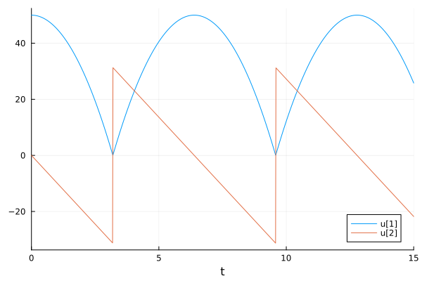

As you can see from the resulting image, DifferentialEquations.jl is smart enough to use the interpolation to hone in on the time of the event and apply the event back at the correct time. Thus, one does not have to worry about the adaptive timestepping “overshooting” the event, as this is handled for you. Notice that the event macro will save the value(s) at the discontinuity.

The callback is robust to having multiple discontinuities occur. For example, we can integrate for long time periods and get the desired behavior:

u0 = [50.0, 0.0]
tspan = (0.0, 100.0)
prob = DE.ODEProblem(f, u0, tspan, p)
sol = DE.solve(prob, DE.Tsit5(), callback = cb)
plot(sol)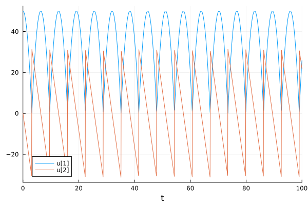

Handling Changing Dynamics and Exactness

Let's make a version of the bouncing ball where the ball sticks to the ground. We can do this by introducing a parameter p to send the velocity to zero on the bounce. This looks as follows:

function dynamics!(du, u, p, t)
    du[1] = u[2]
    du[2] = p[1] * -9.8
    return
end
function floor_aff!(int)
    int.p[1] = 0
    int.u[2] = 0
    return @show int.u[1], int.t
end
floor_event = DE.ContinuousCallback(condition, floor_aff!)
u0 = [1.0, 0.0]
p = [1.0]
prob = DE.ODEProblem{true}(dynamics!, u0, (0.0, 1.75), p)
sol = DE.solve(prob, DE.Tsit5(), callback = floor_event)
plot(sol)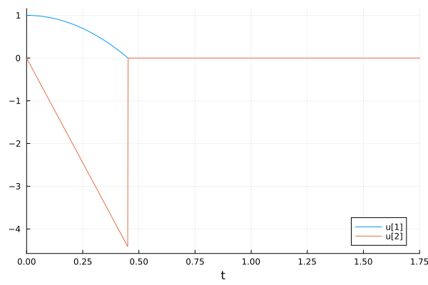

Notice that at the end, the ball is not at 0.0 like the condition would let you believe, but instead it's at 4.329177480185359e-16. From the printing inside the affect function, we can see that this is the value it had at the event time t=0.4517539514526232. Why did the event handling not make it exactly zero? If you instead had run the simulation to nextfloat(0.4517539514526232) = 0.45175395145262326, we would see that the value of u[1] = -1.2647055847076505e-15. You can see this by changing the rootfind argument of the callback:

import SciMLBase
floor_event = DE.ContinuousCallback(condition, floor_aff!, rootfind = SciMLBase.RightRootFind)
u0 = [1.0, 0.0]
p = [1.0]
prob = DE.ODEProblem{true}(dynamics!, u0, (0.0, 1.75), p)
sol = DE.solve(prob, DE.Tsit5(), callback = floor_event)
sol.u[end] # [-1.2647055847076505e-15, 0.0]

2-element Vector{Float64}:
 -2.6988570698778834e-16
  0.0

What this means is that there is no 64-bit floating-point number t such that the condition is zero! By default, if there is no t such that condition=0, then the rootfinder defaults to choosing the floating-point number exactly before the event (LeftRootFind). This way manifold constraints are preserved by default (i.e. the ball never goes below the floor). However, if you require that the condition is exactly satisfied after the event, you will want to add such a change to the affect! function. For example, the error correction in this case is to add int.u[1] = 0 to the affect!, i.e.:

function floor_aff!(int)
    int.p[1] = 0
    int.u[1] = 0
    int.u[2] = 0
    @show int.u[1], int.t
    return
end
floor_event = DE.ContinuousCallback(condition, floor_aff!)
u0 = [1.0, 0.0]
p = [1.0]
prob = DE.ODEProblem{true}(dynamics!, u0, (0.0, 1.75), p)
sol = DE.solve(prob, DE.Tsit5(), callback = floor_event)
sol.u[end] # [0.0,0.0]

2-element Vector{Float64}:
 0.0
 0.0

and now the sticky behavior is perfect to the floating-point.

Handling Accumulation Points

Now let's take a look at the bouncing ball with friction. After the bounce, we will send the velocity to -v/2. Since the velocity is halving each time, we should have Zeno-like behavior and see an accumulation point of bounces. We will use some extra parameters to count the number of bounces (to infinity) and find the accumulation point. Let's watch!

function dynamics!(du, u, p, t)
    du[1] = u[2]
    du[2] = -9.8
    return
end
function floor_aff!(int)
    int.u[2] *= -0.5
    int.p[1] += 1
    int.p[2] = int.t
    return
end
floor_event = DE.ContinuousCallback(condition, floor_aff!)
u0 = [1.0, 0.0]
p = [0.0, 0.0]
prob = DE.ODEProblem{true}(dynamics!, u0, (0.0, 2.0), p)
sol = DE.solve(prob, DE.Tsit5(), callback = floor_event)
plot(sol)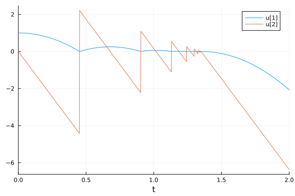

From the readout, we can see the ball only bounced 8 times before it went below the floor, what happened? What happened is floating-point error. Because one cannot guarantee that floating-point numbers exist to make the condition=0, a heuristic is used to ensure that a zero is not accidentally detected at nextfloat(t) after the simulation restarts (otherwise it would repeatedly find the same event!). However, sooner or later, the ability to detect minute floating point differences will crash, and what should be infinitely many bounces finally misses a bounce.

This leads to two questions:

1. How can you improve the accuracy of an accumulation calculation?
2. How can you make it gracefully continue?

For (1), note that floating-point accuracy is dependent on the current dt. If you know that an accumulation point is coming, one can use set_proposed_dt! to shrink the dt value and help find the next bounce point. You can use t - tprev to know the length of the previous interval for this calculation. For this example, we can set the proposed dt to (t - tprev)/10 to ensure an ever-increasing accuracy of the check.

However, at some point we will hit machine epsilon, the value where t + eps(t) == t, so we cannot measure infinitely many bounces and instead will be limited by the floating-point accuracy of our number representation. Using alternative number types like ArbNumerics.jl can allow for this to be done at very high accuracy, but still not infinite. Thus, what we need to do is determine a tolerance after which we assume the accumulation has been reached and define the exit behavior. In this case, we will say when the dt<1e-12, we are almost at the edge of Float64 accuracy (eps(1.0) = 2.220446049250313e-16), so we will change the position and velocity to exactly zero.

With these floating-point corrections in mind, the accumulation calculation looks as follows:

function dynamics!(du, u, p, t)
    du[1] = u[2]
    du[2] = p[1] * -9.8
    return
end
function floor_aff!(int)
    int.u[2] *= -0.5
    if int.dt > 1.0e-12
        DE.set_proposed_dt!(int, (int.t - int.tprev) / 100)
    else
        int.u[1] = 0
        int.u[2] = 0
        int.p[1] = 0
    end
    int.p[2] += 1
    int.p[3] = int.t
    return
end
floor_event = DE.ContinuousCallback(condition, floor_aff!)
u0 = [1.0, 0.0]
p = [1.0, 0.0, 0.0]
prob = DE.ODEProblem{true}(dynamics!, u0, (0.0, 2.0), p)
sol = DE.solve(prob, DE.Tsit5(), callback = floor_event)
plot(sol)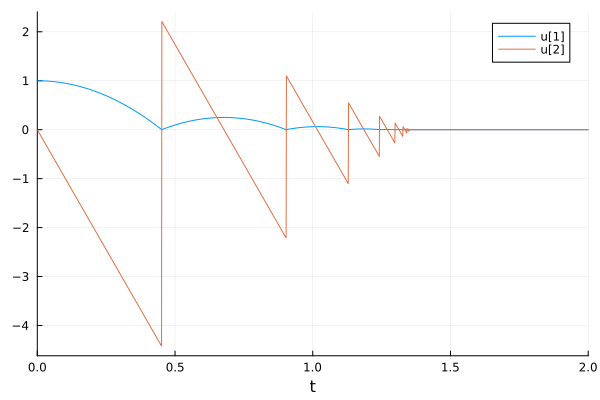

With this corrected version, we see that after 41 bounces, the accumulation point is reached at t = 1.355261854357056. To really see the accumulation, let's zoom in:

p1 = plot(sol, idxs = 1, tspan = (1.25, 1.4))
p2 = plot(sol, idxs = 1, tspan = (1.35, 1.36))
p3 = plot(sol, idxs = 1, tspan = (1.354, 1.35526))
p4 = plot(sol, idxs = 1, tspan = (1.35526, 1.35526185))
plot(p1, p2, p3, p4)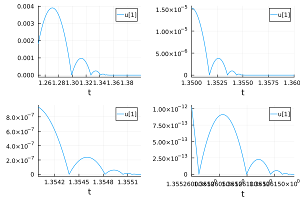

I think Zeno would be proud of our solution.

Example 2: Terminating an Integration

Often, you might want to terminate an integration when some condition is satisfied. To terminate an integration, use terminate!(integrator) as the affect! in a callback.

In this example, we will solve the differential equation:

import DifferentialEquations as DE
u0 = [1.0, 0.0]
function fun2(du, u, p, t)
    du[2] = -u[1]
    du[1] = u[2]
    return
end
tspan = (0.0, 10.0)
prob = DE.ODEProblem(fun2, u0, tspan)

ODEProblem with uType Vector{Float64} and tType Float64. In-place: true
Non-trivial mass matrix: false
timespan: (0.0, 10.0)
u0: 2-element Vector{Float64}:
 1.0
 0.0

which has cosine and -sine as the solutions respectively. We wish to solve until the sine part, u[2] becomes positive. There are two things we may be looking for.

A DiscreteCallback will cause this to halt at the first step such that the condition is satisfied. For example, we could use:

condition(u, t, integrator) = u[2] > 0
affect!(integrator) = DE.terminate!(integrator)
cb = DE.DiscreteCallback(condition, affect!)
sol = DE.solve(prob, DE.Tsit5(), callback = cb)

retcode: Terminated
Interpolation: specialized 4th order "free" interpolation
t: 13-element Vector{Float64}:
 0.0
 0.0009990009990009992
 0.027576749618897903
 0.13188573886863814
 0.3267494406221896
 0.5929469647213219
 0.9349025596193421
 1.3541389472147036
 1.8251515994880871
 2.2911636620830027
 2.887283753877988
 3.508600087718049
 3.508600087718049
u: 13-element Vector{Vector{Float64}}:
 [1.0, 0.0]
 [0.9999995009985435, -0.000999000832833342]
 [0.9996197855364959, -0.027573254503947372]
 [0.9913156746593331, -0.131503737850086]
 [0.9470906620351799, -0.3209661568511073]
 [0.8292974726417712, -0.5588073699912273]
 [0.5938966746905806, -0.8045412656131483]
 [0.21496568103479724, -0.9766215020180059]
 [-0.2516232076244374, -0.9678251582901]
 [-0.6596628721252128, -0.7515614599792891]
 [-0.9678404150581446, -0.2515685294370578]
 [-0.9334019218518724, 0.35883967708678305]
 [-0.9334019218518724, 0.35883967708678305]

However, we often wish to halt exactly at the point of time that the condition is satisfied. To achieve that, we use a continuous callback. The condition must thus be a function which is zero at the point we want to halt. Thus, we use the following:

condition(u, t, integrator) = u[2]
affect!(integrator) = DE.terminate!(integrator)
cb = DE.ContinuousCallback(condition, affect!)
sol = DE.solve(prob, DE.Tsit5(), callback = cb)
import Plots: plot
plot(sol);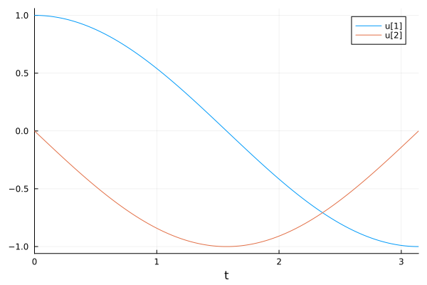

Note that this uses rootfinding to approximate the “exact” moment of the crossing. Analytically we know the value is pi, and here the integration terminates at

sol.t[end] # 3.1415902502224307

3.141580646344477

Using a more accurate integration increases the accuracy of this prediction:

sol = DE.solve(prob, DE.Vern8(), callback = cb, reltol = 1.0e-12, abstol = 1.0e-12)
#π = 3.141592653589703...
sol.t[end] # 3.1415926535896035

3.1415926535784626

Now say we wish to find when the first period is over, i.e. we want to ignore the upcrossing and only stop on the downcrossing. We do this by ignoring the affect! and only passing an affect! for the second:

condition(u, t, integrator) = u[2]
affect!(integrator) = DE.terminate!(integrator)
cb = DE.ContinuousCallback(condition, nothing, affect!)
sol = DE.solve(prob, DE.Tsit5(), callback = cb)
plot(sol)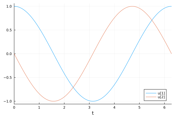

Notice that passing only one affect! is the same as ContinuousCallback(condition,affect!,affect!), i.e. both upcrossings and downcrossings will activate the event. Using ContinuousCallback(condition,affect!,nothing)will thus be the same as above because the first event is an upcrossing.

Example 3: Growing Cell Population

Another interesting issue is with models of changing sizes. The ability to handle such events is a unique feature of DifferentialEquations.jl! The problem we would like to tackle here is a cell population. We start with 1 cell with a protein X which increases linearly with time with rate parameter α. Since we will be changing the size of the population, we write the model in the general form:

const α = 0.3
function f(du, u, p, t)
    for i in 1:length(u)
        du[i] = α * u[i]
    end
    return
end

f (generic function with 1 method)

Our model is that, whenever the protein X gets to a concentration of 1, it triggers a cell division. So we check to see if any concentrations hit 1:

# Event when condition(u,t,integrator) == 0
condition(u, t, integrator) = 1 - maximum(u)

condition (generic function with 1 method)

Again, recall that this function finds events as when condition==0, so 1-maximum(u) is positive until a cell has a concentration of X which is 1, which then triggers the event. At the event, we have that the cell splits into two cells, giving a random amount of protein to each one. We can do this by resizing the cache (adding 1 to the length of all of the caches) and setting the values of these two cells at the time of the event:

function affect!(integrator)
    u = integrator.u
    maxidx = findmax(u)[2]
    resize!(integrator, length(u) + 1)
    Θ = rand()
    u[maxidx] = Θ
    u[end] = 1 - Θ
    return
end

affect! (generic function with 1 method)

As noted in the Integrator Interface, resize!(integrator,length(integrator.u)+1) is used to change the length of all of the internal caches (which includes u) to be their current length + 1, growing the ODE system. Then the following code sets the new protein concentrations. Now we can solve:

import DifferentialEquations as DE
callback = DE.ContinuousCallback(condition, affect!)
u0 = [0.2]
tspan = (0.0, 10.0)
prob = DE.ODEProblem(f, u0, tspan)
sol = DE.solve(prob; callback)

retcode: Success
Interpolation: 3rd order Hermite
t: 22-element Vector{Float64}:
  0.0
  0.12735293592636002
  0.7397598133657947
  1.7483495107714813
  2.946671013454737
  4.439320780532288
  5.364806632471663
  5.364806632471663
  5.942782519689807
  5.942782519689807
  ⋮
  8.802769677938947
  8.802769677938947
  9.079377137669702
  9.079377137669702
  9.567539135883603
  9.567539135883603
  9.699985759530751
  9.699985759530751
 10.0
u: 22-element Vector{Vector{Float64}}:
 [0.2]
 [0.20778902193773555]
 [0.24969628285979079]
 [0.3379244024793189]
 [0.48411312693417946]
 [0.7575679841004618]
 [0.999999999999999]
 [0.15919284791065957, 0.8408071520893404]
 [0.1893333655821999, 0.9999999999999999]
 [0.1893333655821999, 0.5759850400873087, 0.42401495991269134]
 ⋮
 [0.4465252018966159, 0.5634216142424314, 0.9999999999999992, 0.7949857405497424]
 [0.4465252018966159, 0.5634216142424314, 0.9203672002997826, 0.7949857405497424, 0.07963279970021742]
 [0.4851598381071961, 0.6121704620274532, 1.0, 0.8637701781319445, 0.08652285704475272]
 [0.4851598381071961, 0.6121704620274532, 0.38305246517298275, 0.8637701781319445, 0.08652285704475272, 0.6169475348270173]
 [0.561676995096589, 0.7087191448903455, 0.44346572140450746, 0.9999999999999998, 0.10016884031800409, 0.7142496354311225]
 [0.561676995096589, 0.7087191448903455, 0.44346572140450746, 0.03895494785503539, 0.10016884031800409, 0.7142496354311225, 0.9610450521449646]
 [0.5844439798560715, 0.7374463281492883, 0.46144113682780274, 0.04053394559192778, 0.10422907864146057, 0.7432009912927419, 1.0]
 [0.5844439798560715, 0.7374463281492883, 0.46144113682780274, 0.04053394559192778, 0.10422907864146057, 0.7432009912927419, 0.15061701524320814, 0.8493829847567919]
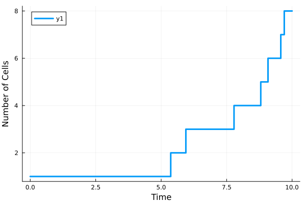
 [0.6394863050023706, 0.806898255059261, 0.5048991823626522, 0.0443513903593163, 0.1140452646815585, 0.8131948863823294, 0.16480196882528347, 0.9293769893699126]

The plot recipes do not have a way of handling the changing size, but we can plot from the solution object directly. For example, let's make a plot of how many cells there are at each time. Since these are discrete values, we calculate and plot them directly:

import Plots: plot
plot(
    sol.t, map(length, sol[:]), lw = 3,
    ylabel = "Number of Cells", xlabel = "Time"
)

Now let's check in on a cell. We can still use the interpolation to get a nice plot of the concentration of cell 1 over time. This is done with the command:

ts = range(0, stop = 10, length = 100)
plot(
    ts, map(first, sol.(ts)), lw = 3,
    ylabel = "Amount of X in Cell 1", xlabel = "Time"
)

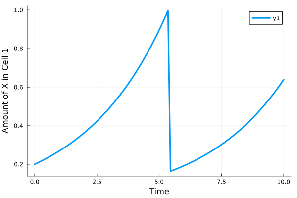
Notice that every time it hits 1 the cell divides, giving cell 1 a random amount of X which then grows until the next division.

Note that one macro which was not shown in this example is deleteat! on the caches. For example, to delete the second cell, we could use:

DE.deleteat!(integrator, 2)

This allows you to build sophisticated models of populations with births and deaths.

VectorContinuousCallback Example

Example 1: Bouncing Ball with multiple walls

This is similar to the above Bouncing Ball example, but now we have two more vertical walls, at x = 0 and x = 10.0. We have our ODEFunction as -

function f(du, u, p, t)
    du[1] = u[2]
    du[2] = -p
    du[3] = u[4]
    du[4] = 0.0
    return
end

f (generic function with 1 method)

where u[1] denotes y-coordinate, u[2] denotes velocity in y-direction, u[3] denotes x-coordinate and u[4] denotes velocity in x-direction. We will make a VectorContinuousCallback of length 2 - one for x axis collision, one for walls parallel to y axis.

function condition(out, u, t, integrator) # Event when condition(out,u,t,integrator) == 0
    out[1] = u[1]
    out[2] = (u[3] - 10.0)u[3]
    return
end

function affect!(integrator, idx)
    if idx == 1
        integrator.u[2] = -0.9integrator.u[2]
    elseif idx == 2
        integrator.u[4] = -0.9integrator.u[4]
    end
    return
end
import DifferentialEquations as DE
cb = DE.VectorContinuousCallback(condition, affect!, 2)

VectorContinuousCallback{typeof(Main.condition), typeof(Main.affect!), typeof(SciMLBase.INITIALIZE_DEFAULT), typeof(SciMLBase.FINALIZE_DEFAULT), Float64, Int64, Rational{Int64}, Nothing, Nothing, Int64, Tuple{}}(Main.condition, Main.affect!, 2, SciMLBase.INITIALIZE_DEFAULT, SciMLBase.FINALIZE_DEFAULT, nothing, LeftRootFind, 10, Bool[1, 1], 1, 2.220446049250313e-15, 0, 1//100, nothing, (), true, true)

It is evident that out[2] will be zero when u[3] (x-coordinate) is either 0.0 or 10.0. And when that happens, we flip the velocity with some coefficient of restitution (0.9).

Completing the rest of the code

u0 = [50.0, 0.0, 0.0, 2.0]
tspan = (0.0, 15.0)
p = 9.8
prob = DE.ODEProblem(f, u0, tspan, p)
sol = DE.solve(prob, DE.Tsit5(), callback = cb, dt = 1.0e-3, adaptive = false)
import Plots: plot
plot(sol, idxs = (1, 3));