Automated Efficient Solution of Nonlinear Partial Differential Equations
Solving nonlinear partial differential equations (PDEs) is hard. Solving nonlinear PDEs fast and accurately is even harder. Doing it all in an automated method from just a symbolic description is just plain fun. That's what we'd demonstrate here: how to solve a nonlinear PDE from a purely symbolic definition using the combination of ModelingToolkit, MethodOfLines, and DifferentialEquations.jl.
This example is a combination of the Brusselator tutorial from MethodOfLines.jl and the Solving Large Stiff Equations tutorial from DifferentialEquations.jl.
Required Dependencies
The following parts of the SciML Ecosystem will be used in this tutorial:
| Module | Description |
|---|---|
| ModelingToolkit.jl | The symbolic modeling environment |
| MethodOfLines.jl | The symbolic PDE discretization tooling |
| DifferentialEquations.jl | The numerical differential equation solvers |
Problem Setup
The Brusselator PDE is defined as follows:
\[\begin{align} \frac{\partial u}{\partial t} &= 1 + u^2v - 4.4u + \alpha \left(\frac{\partial^2 u}{\partial x^2} + \frac{\partial^2 u}{\partial y^2}\right) + f(x, y, t)\\ \frac{\partial v}{\partial t} &= 3.4u - u^2v + \alpha \left(\frac{\partial^2 v}{\partial x^2} + \frac{\partial^2 v}{\partial y^2}\right) \end{align}\]
where
\[f(x, y, t) = \begin{cases} 5 & \quad \text{if } (x-0.3)^2+(y-0.6)^2 ≤ 0.1^2 \text{ and } t ≥ 1.1 \\ 0 & \quad \text{else} \end{cases}\]
and the initial conditions are
\[\begin{align} u(x, y, 0) &= 22\cdot (y(1-y))^{3/2} \\ v(x, y, 0) &= 27\cdot (x(1-x))^{3/2} \end{align}\]
with the periodic boundary condition
\[\begin{align} u(x+1,y,t) &= u(x,y,t) \\ u(x,y+1,t) &= u(x,y,t) \end{align}\]
We wish to obtain the solution to this PDE on a timespan of $t \in [0,11.5]$.
Defining the symbolic PDEsystem with ModelingToolkit.jl
With ModelingToolkit.jl, we first symbolically define the system, see also the docs for PDESystem:
import MethodOfLines
import OrdinaryDiffEq as ODE
import SciMLBase
import DomainSets: Interval
using ModelingToolkit: @named, @parameters, @variables, Differential, PDESystem

@parameters x y t
@variables u(..) v(..)
Dt = Differential(t)
Dx = Differential(x)
Dy = Differential(y)
Dxx = Differential(x)^2
Dyy = Differential(y)^2

∇²(u) = Dxx(u) + Dyy(u)

brusselator_f(x, y, t) = (((x - 0.3)^2 + (y - 0.6)^2) <= 0.1^2) * (t >= 1.1) * 5.0

x_min = y_min = t_min = 0.0
x_max = y_max = 1.0
t_max = 11.5

α = 10.0

u0(x, y, t) = 22(y * (1 - y))^(3 / 2)
v0(x, y, t) = 27(x * (1 - x))^(3 / 2)

eq = [
    Dt(u(x, y, t)) ~ 1.0 + v(x, y, t) * u(x, y, t)^2 - 4.4 * u(x, y, t) +
        α * ∇²(u(x, y, t)) + brusselator_f(x, y, t),
    Dt(v(x, y, t)) ~ 3.4 * u(x, y, t) - v(x, y, t) * u(x, y, t)^2 + α * ∇²(v(x, y, t)),
]

domains = [
    x ∈ Interval(x_min, x_max),
    y ∈ Interval(y_min, y_max),
    t ∈ Interval(t_min, t_max),
]

# Periodic BCs
bcs = [
    u(x, y, 0) ~ u0(x, y, 0),
    u(0, y, t) ~ u(1, y, t),
    u(x, 0, t) ~ u(x, 1, t), v(x, y, 0) ~ v0(x, y, 0),
    v(0, y, t) ~ v(1, y, t),
    v(x, 0, t) ~ v(x, 1, t),
]

@named pdesys = PDESystem(eq, bcs, domains, [x, y, t], [u(x, y, t), v(x, y, t)])
\[ \begin{align} \frac{\mathrm{d}}{\mathrm{d}t} ~ u\left( x, y, t \right) &= 1 + 10 ~ \left( \frac{\mathrm{d}^{2}}{\mathrm{d}x^{2}} ~ u\left( x, y, t \right) + \frac{\mathrm{d}^{2}}{\mathrm{d}y^{2}} ~ u\left( x, y, t \right) \right) - 4.4 ~ u\left( x, y, t \right) + 5 ~ \left( \left( -0.3 + x \right)^{2} + \left( -0.6 + y \right)^{2} \leq 0.01 \right) ~ \left( t \geq 1.1 \right) + \left( u\left( x, y, t \right) \right)^{2} ~ v\left( x, y, t \right) \\ \frac{\mathrm{d}}{\mathrm{d}t} ~ v\left( x, y, t \right) &= 10 ~ \left( \frac{\mathrm{d}^{2}}{\mathrm{d}y^{2}} ~ v\left( x, y, t \right) + \frac{\mathrm{d}^{2}}{\mathrm{d}x^{2}} ~ v\left( x, y, t \right) \right) + 3.4 ~ u\left( x, y, t \right) - \left( u\left( x, y, t \right) \right)^{2} ~ v\left( x, y, t \right) \end{align} \]
Looks just like the LaTeX description, right? Now let's solve it.
Automated symbolic discretization with MethodOfLines.jl
Next we create the discretization. Here we will use the finite difference method via method of lines. Method of lines is a method of recognizing that a discretization of a partial differential equation transforms it into a new numerical problem. For example:
| Discretization Form | Numerical Problem Type |
|---|---|
| Finite Difference, Finite Volume, Finite Element, discretizing all variables | NonlinearProblem |
| MethodOfLines finite differences, discretizing all variables except time | Array-form DAEProblem |
| Physics-Informed Neural Network | OptimizationProblem |
| Feynman-Kac Formula | SDEProblem |
| Universal Stochastic Differential Equation (High dimensional PDEs) | OptimizationProblem inverse problem over SDEProblem |
Thus the process of solving a PDE is fundamentally about transforming its symbolic form to a standard numerical problem and solving the standard numerical problem using one of the solvers in the SciML ecosystem! Here we will demonstrate one of the most classic methods: the finite difference method. Since the Brusselator is a time-dependent PDE with heavy stiffness in the time domain, we will leave time undiscretized. MethodOfLines discretizes the x and y domains while representing operations over the complete arrays of grid values. The result is a differential-algebraic equation (DAE) for how those values evolve over time.
To do this, we use the MOLFiniteDifference construct of MethodOfLines.jl as follows:
N = 32

dx = (x_max - x_min) / N
dy = (y_max - y_min) / N

order = 2

discretization = MethodOfLines.MOLFiniteDifference(
    [x => dx, y => dy], t, approx_order = order,
    grid_align = MethodOfLines.center_align
)
MethodOfLines.MOLFiniteDifference{MethodOfLines.CenterAlignedGrid}(Dict{Symbolics.Num, Float64}(x => 0.03125, y => 0.03125), t, 2, MethodOfLines.UpwindScheme(1), MethodOfLines.CenterAlignedGrid(), true, true, Any[], Base.Pairs{Symbol, Union{}, Tuple{}, @NamedTuple{}}())Next, we discretize the system. MethodOfLines v1 constructs an array-form DAEProblem for supported time-dependent systems. The fallback = false keyword enforces that array form so this tutorial fails if the PDE is not supported by it:
prob = MethodOfLines.discretize(pdesys, discretization; fallback = false)
@assert prob isa SciMLBase.DAEProblem
┌ Warning: The system contains interface boundaries, which are not compatible with system transformation. The system will not be transformed. Please post an issue if you need this feature.
└ @ MethodOfLines ~/.julia/packages/MethodOfLines/tt4Yz/src/system_parsing/pde_system_transformation.jl:55The symbolic equations operate on whole array slices rather than generating one scalar equation per grid point. For a fixed PDE system, this keeps symbolic compilation independent of the spatial grid size. Discretization, storage, and numerical solution still scale with the number of grid points.
Solving the PDE
Calling solve without an explicit algorithm lets OrdinaryDiffEq select its default DAE solver and preserves the array-form compilation path:
sol = ODE.solve(prob; saveat = 0.1);retcode: Success
Interpolation: Dict{Symbolics.Num, Interpolations.GriddedInterpolation{Float64, 3, Array{Float64, 3}, Interpolations.Gridded{Interpolations.Linear{Interpolations.Throw{Interpolations.OnGrid}}}, Tuple{Vector{Float64}, Vector{Float64}, Vector{Float64}}}}
t: 116-element Vector{Float64}:
0.0
0.1
0.2
0.3
0.4
0.5
0.6
0.7
0.8
0.9
⋮
10.7
10.8
10.9
11.0
11.1
11.2
11.3
11.4
11.5ivs: 3-element Vector{SymbolicUtils.BasicSymbolicImpl.var"typeof(BasicSymbolicImpl)"{SymbolicUtils.SymReal}}:
t
x
ydomain:([0.0, 0.1, 0.2, 0.3, 0.4, 0.5, 0.6, 0.7, 0.8, 0.9 … 10.6, 10.7, 10.8, 10.9, 11.0, 11.1, 11.2, 11.3, 11.4, 11.5], 0.0:0.03125:1.0, 0.0:0.03125:1.0)
u: Dict{Symbolics.Num, Array{Float64, 3}} with 2 entries:
u(x, y, t) => [0.0 0.115882 … 0.115882 0.0; 0.0 0.115882 … 0.115882 0.0; … ; …
v(x, y, t) => [0.0 0.0 … 0.0 0.0; 0.142219 0.142219 … 0.142219 0.142219; … ; …Examining Results via the Symbolic Solution Interface
Now that we have solved the DAE representation of the PDE, we have a PDETimeSeriesSolution that wraps the numerical DAE solution, which we can get with sol.original_sol. The raw solver state stores the grid values in its numerical ordering, but that ordering is not the most useful way to interpret a PDE solution.
To make the handling of such cases a lot simpler, MethodOfLines.jl implements a symbolic interface for the solution object that allows for interpreting the computation through its original representation. For example, if we want to know how to interpret the values of the grid corresponding to the independent variables, we can just index using symbolic variables:
discrete_x = sol[x];
discrete_y = sol[y];
discrete_t = sol[t];
116-element Vector{Float64}:
0.0
0.1
0.2
0.3
0.4
0.5
0.6
0.7
0.8
0.9
⋮
10.7
10.8
10.9
11.0
11.1
11.2
11.3
11.4
11.5What this tells us is that, for a solution at a given time point, say original_sol[1] for the solution at the initial time (the initial condition), the value original_sol[1][1] is the solution at the grid point (discrete_x[1], discrete_y[1]). For values that are not the initial time point, original_sol[i] corresponds to the solution at discrete_t[i].
But we also have two dependent variables, u and v. How do we interpret which of the results correspond to the different dependent variables? This is done by indexing the solution by the dependent variables! For example:
solu = sol[u(x, y, t)];
solv = sol[v(x, y, t)];
33×33×116 Array{Float64, 3}:
[:, :, 1] =
0.0 0.0 0.0 0.0 … 0.0 0.0 0.0
0.142219 0.142219 0.142219 0.142219 0.142219 0.142219 0.142219
0.382949 0.382949 0.382949 0.382949 0.382949 0.382949 0.382949
0.668641 0.668641 0.668641 0.668641 0.668641 0.668641 0.668641
0.976654 0.976654 0.976654 0.976654 0.976654 0.976654 0.976654
1.29245 1.29245 1.29245 1.29245 … 1.29245 1.29245 1.29245
1.60546 1.60546 1.60546 1.60546 1.60546 1.60546 1.60546
1.90753 1.90753 1.90753 1.90753 1.90753 1.90753 1.90753
2.19213 2.19213 2.19213 2.19213 2.19213 2.19213 2.19213
2.45397 2.45397 2.45397 2.45397 2.45397 2.45397 2.45397
⋮ ⋱ ⋮
2.19213 2.19213 2.19213 2.19213 2.19213 2.19213 2.19213
1.90753 1.90753 1.90753 1.90753 … 1.90753 1.90753 1.90753
1.60546 1.60546 1.60546 1.60546 1.60546 1.60546 1.60546
1.29245 1.29245 1.29245 1.29245 1.29245 1.29245 1.29245
0.976654 0.976654 0.976654 0.976654 0.976654 0.976654 0.976654
0.668641 0.668641 0.668641 0.668641 0.668641 0.668641 0.668641
0.382949 0.382949 0.382949 0.382949 … 0.382949 0.382949 0.382949
0.142219 0.142219 0.142219 0.142219 0.142219 0.142219 0.142219
0.0 0.0 0.0 0.0 0.0 0.0 0.0
[:, :, 2] =
0.0 2.02429 2.02429 2.02429 … 2.02429 2.02429 2.02429 2.02429
2.02429 2.02429 2.02429 2.02429 2.02429 2.02429 2.02429 2.02429
2.02429 2.02429 2.02429 2.02429 2.02429 2.02429 2.02429 2.02429
2.02429 2.02429 2.02429 2.02429 2.02429 2.02429 2.02429 2.02429
2.0243 2.0243 2.0243 2.0243 2.0243 2.0243 2.0243 2.0243
2.0243 2.0243 2.0243 2.0243 … 2.0243 2.0243 2.0243 2.0243
2.02431 2.02431 2.02431 2.02431 2.02431 2.02431 2.02431 2.02431
2.02432 2.02432 2.02432 2.02432 2.02432 2.02432 2.02432 2.02432
2.02433 2.02433 2.02433 2.02433 2.02433 2.02433 2.02433 2.02433
2.02433 2.02433 2.02433 2.02433 2.02433 2.02433 2.02433 2.02433
⋮ ⋱ ⋮
2.02433 2.02433 2.02433 2.02433 2.02433 2.02433 2.02433 2.02433
2.02432 2.02432 2.02432 2.02432 … 2.02432 2.02432 2.02432 2.02432
2.02431 2.02431 2.02431 2.02431 2.02431 2.02431 2.02431 2.02431
2.0243 2.0243 2.0243 2.0243 2.0243 2.0243 2.0243 2.0243
2.0243 2.0243 2.0243 2.0243 2.0243 2.0243 2.0243 2.0243
2.02429 2.02429 2.02429 2.02429 2.02429 2.02429 2.02429 2.02429
2.02429 2.02429 2.02429 2.02429 … 2.02429 2.02429 2.02429 2.02429
2.02429 2.02429 2.02429 2.02429 2.02429 2.02429 2.02429 2.02429
2.02429 2.02429 2.02429 2.02429 2.02429 2.02429 2.02429 2.02429
[:, :, 3] =
0.0 2.07964 2.07964 2.07964 … 2.07964 2.07964 2.07964 2.07964
2.07964 2.07964 2.07964 2.07964 2.07964 2.07964 2.07964 2.07964
2.07964 2.07964 2.07964 2.07964 2.07964 2.07964 2.07964 2.07964
2.07964 2.07964 2.07964 2.07964 2.07964 2.07964 2.07964 2.07964
2.07964 2.07964 2.07964 2.07964 2.07964 2.07964 2.07964 2.07964
2.07964 2.07964 2.07964 2.07964 … 2.07964 2.07964 2.07964 2.07964
2.07964 2.07964 2.07964 2.07965 2.07965 2.07964 2.07964 2.07964
2.07964 2.07964 2.07965 2.07965 2.07965 2.07965 2.07964 2.07964
2.07965 2.07965 2.07965 2.07965 2.07965 2.07965 2.07965 2.07965
2.07965 2.07965 2.07965 2.07965 2.07965 2.07965 2.07965 2.07965
⋮ ⋱ ⋮
2.07965 2.07965 2.07965 2.07965 2.07965 2.07965 2.07965 2.07965
2.07964 2.07964 2.07965 2.07965 … 2.07965 2.07965 2.07964 2.07964
2.07964 2.07964 2.07964 2.07965 2.07965 2.07964 2.07964 2.07964
2.07964 2.07964 2.07964 2.07964 2.07964 2.07964 2.07964 2.07964
2.07964 2.07964 2.07964 2.07964 2.07964 2.07964 2.07964 2.07964
2.07964 2.07964 2.07964 2.07964 2.07964 2.07964 2.07964 2.07964
2.07964 2.07964 2.07964 2.07964 … 2.07964 2.07964 2.07964 2.07964
2.07964 2.07964 2.07964 2.07964 2.07964 2.07964 2.07964 2.07964
2.07964 2.07964 2.07964 2.07964 2.07964 2.07964 2.07964 2.07964
;;; …
[:, :, 114] =
0.0 3.95161 3.95161 3.95161 … 3.9516 3.9516 3.95161 3.95161
3.95161 3.95161 3.95161 3.95161 3.9516 3.9516 3.9516 3.95161
3.9516 3.95161 3.95161 3.95161 3.9516 3.9516 3.9516 3.9516
3.9516 3.9516 3.9516 3.95161 3.95159 3.9516 3.9516 3.9516
3.9516 3.9516 3.9516 3.9516 3.95159 3.95159 3.9516 3.9516
3.9516 3.9516 3.9516 3.9516 … 3.95159 3.95159 3.95159 3.9516
3.95159 3.9516 3.9516 3.9516 3.95158 3.95159 3.95159 3.95159
3.95159 3.9516 3.9516 3.9516 3.95158 3.95159 3.95159 3.95159
3.95159 3.95159 3.9516 3.9516 3.95158 3.95158 3.95159 3.95159
3.95159 3.95159 3.9516 3.9516 3.95158 3.95158 3.95159 3.95159
⋮ ⋱ ⋮
3.95162 3.95162 3.95162 3.95162 3.95161 3.95161 3.95162 3.95162
3.95162 3.95162 3.95162 3.95162 … 3.95161 3.95161 3.95162 3.95162
3.95162 3.95162 3.95162 3.95162 3.95161 3.95161 3.95162 3.95162
3.95162 3.95162 3.95162 3.95162 3.95161 3.95161 3.95162 3.95162
3.95162 3.95162 3.95162 3.95162 3.95161 3.95161 3.95161 3.95162
3.95162 3.95162 3.95162 3.95162 3.95161 3.95161 3.95161 3.95162
3.95161 3.95161 3.95162 3.95162 … 3.95161 3.95161 3.95161 3.95161
3.95161 3.95161 3.95161 3.95161 3.9516 3.95161 3.95161 3.95161
3.95161 3.95161 3.95161 3.95161 3.9516 3.9516 3.95161 3.95161
[:, :, 115] =
0.0 3.02211 3.02212 3.02212 … 3.0221 3.02211 3.02211 3.02211
3.02211 3.02211 3.02211 3.02211 3.0221 3.0221 3.02211 3.02211
3.02211 3.02211 3.02211 3.02211 3.0221 3.0221 3.0221 3.02211
3.0221 3.02211 3.02211 3.02211 3.02209 3.0221 3.0221 3.0221
3.0221 3.0221 3.02211 3.02211 3.02209 3.02209 3.0221 3.0221
3.0221 3.0221 3.0221 3.0221 … 3.02209 3.02209 3.0221 3.0221
3.0221 3.0221 3.0221 3.0221 3.02208 3.02209 3.02209 3.0221
3.0221 3.0221 3.0221 3.0221 3.02208 3.02209 3.02209 3.0221
3.02209 3.0221 3.0221 3.0221 3.02208 3.02209 3.02209 3.02209
3.02209 3.0221 3.0221 3.0221 3.02208 3.02209 3.02209 3.02209
⋮ ⋱ ⋮
3.02212 3.02212 3.02213 3.02213 3.02212 3.02212 3.02212 3.02212
3.02212 3.02213 3.02213 3.02213 … 3.02212 3.02212 3.02212 3.02212
3.02212 3.02213 3.02213 3.02213 3.02212 3.02212 3.02212 3.02212
3.02212 3.02212 3.02213 3.02213 3.02212 3.02212 3.02212 3.02212
3.02212 3.02212 3.02212 3.02212 3.02212 3.02212 3.02212 3.02212
3.02212 3.02212 3.02212 3.02212 3.02211 3.02212 3.02212 3.02212
3.02212 3.02212 3.02212 3.02212 … 3.02211 3.02211 3.02212 3.02212
3.02212 3.02212 3.02212 3.02212 3.02211 3.02211 3.02211 3.02212
3.02211 3.02211 3.02212 3.02212 3.0221 3.02211 3.02211 3.02211
[:, :, 116] =
0.0 1.74765 1.74765 1.74765 … 1.74764 1.74764 1.74765 1.74765
1.74764 1.74765 1.74765 1.74765 1.74764 1.74764 1.74764 1.74764
1.74764 1.74764 1.74765 1.74765 1.74763 1.74764 1.74764 1.74764
1.74764 1.74764 1.74764 1.74764 1.74763 1.74764 1.74764 1.74764
1.74764 1.74764 1.74764 1.74764 1.74763 1.74763 1.74764 1.74764
1.74764 1.74764 1.74764 1.74764 … 1.74763 1.74763 1.74763 1.74764
1.74763 1.74764 1.74764 1.74764 1.74762 1.74763 1.74763 1.74763
1.74763 1.74764 1.74764 1.74764 1.74762 1.74763 1.74763 1.74763
1.74763 1.74763 1.74764 1.74764 1.74762 1.74763 1.74763 1.74763
1.74763 1.74763 1.74764 1.74764 1.74762 1.74763 1.74763 1.74763
⋮ ⋱ ⋮
1.74765 1.74766 1.74766 1.74766 1.74765 1.74765 1.74765 1.74765
1.74765 1.74766 1.74766 1.74766 … 1.74765 1.74765 1.74765 1.74765
1.74765 1.74766 1.74766 1.74766 1.74765 1.74765 1.74765 1.74765
1.74765 1.74766 1.74766 1.74766 1.74765 1.74765 1.74765 1.74765
1.74765 1.74765 1.74766 1.74766 1.74765 1.74765 1.74765 1.74765
1.74765 1.74765 1.74765 1.74765 1.74765 1.74765 1.74765 1.74765
1.74765 1.74765 1.74765 1.74765 … 1.74765 1.74765 1.74765 1.74765
1.74765 1.74765 1.74765 1.74765 1.74764 1.74765 1.74765 1.74765
1.74765 1.74765 1.74765 1.74765 1.74764 1.74764 1.74765 1.74765This then gives an array of results for the u and v separately, each dimension corresponding to the discrete form of the independent variables.
Using this high-level indexing, we can create an animation of the solution of the Brusselator as follows. For u we receive:
import Plots
anim = Plots.@animate for k in 1:length(discrete_t)
    Plots.heatmap(solu[2:end, 2:end, k], title = "$(discrete_t[k])") # 2:end since end = 1, periodic condition
end
Plots.gif(anim, "plots/Brusselator2Dsol_u.gif", fps = 8)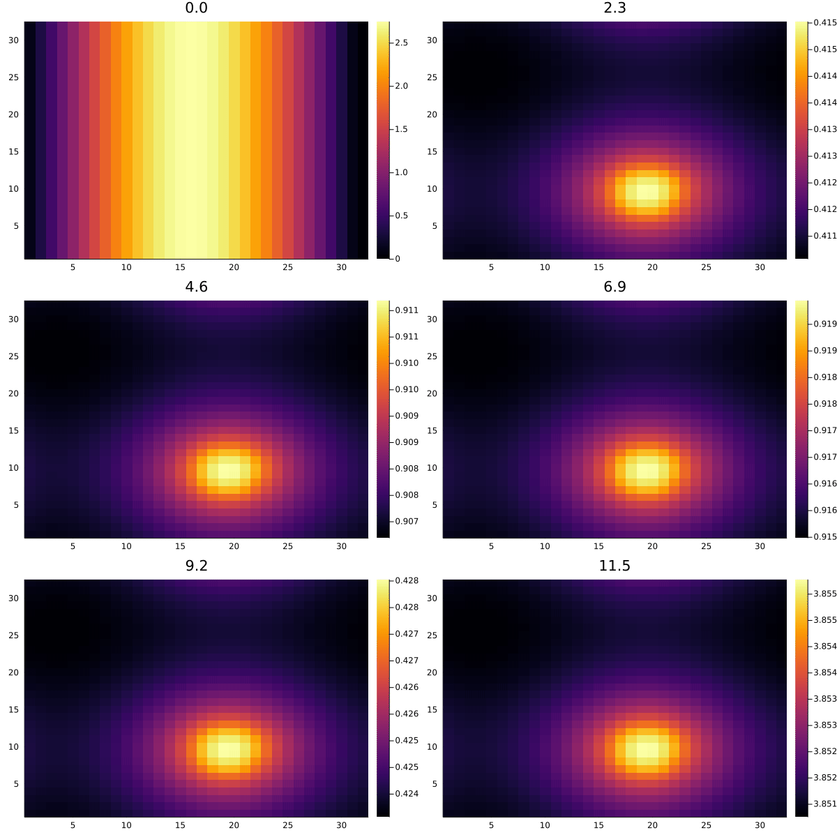
and for v:
anim = Plots.@animate for k in 1:length(discrete_t)
    Plots.heatmap(solv[2:end, 2:end, k], title = "$(discrete_t[k])")
end
Plots.gif(anim, "plots/Brusselator2Dsol_v.gif", fps = 8)
Why Keep the Array-Form DAE?
MethodOfLines keeps the spatial operations as array-slice equations when it constructs the DAEProblem. Code generation therefore follows the array representation instead of generating a separate scalar expression for every grid point. Keep this array-form problem and solve it with a DAE solver to retain grid-independent symbolic compilation.
If you're interested in figuring out what's the fastest current solver for this kind of PDE, check out the Brusselator benchmark in SciMLBenchmarks.jl