Building a model to add to ReservoirComputing.jl

This example showcases how to build custom models that could also be included in ReservoirComputing.jl. In this example we will build an edge-of-stability echo state network (ES2N). ES2N. Since the model is already available in the library, we will change the names of cells and models to avoid conflicts.

Building an ES2NCell

Building a ReservoirComputing.jl model largely follows the Lux.jl model approach.

using ReservoirComputing
using LuxCore
using WeightInitializers
using ConcreteStructs
using Random

import LuxCore: initialparameters, setup

@concrete struct CustomES2NCell <: ReservoirComputing.AbstractEchoStateNetworkCell
    activation
    in_dims <: Integer
    out_dims <: Integer
    init_bias
    init_reservoir
    init_input
    init_orthogonal
    init_state
    proximity
    use_bias::Bool
end

function CustomES2NCell((in_dims, out_dims)::Pair{<:Integer, <:Integer},
        activation = tanh; use_bias::Bool = false, init_bias = zeros32,
        init_reservoir = rand_sparse, init_input = scaled_rand,
        init_state = randn32, init_orthogonal = orthogonal,
        proximity::AbstractFloat = 1.0)
    return CustomES2NCell(activation, in_dims, out_dims, init_bias, init_reservoir,
        init_input, init_orthogonal, init_state, proximity, use_bias)
end

function initialparameters(rng::Random.AbstractRNG, esn::CustomES2NCell)
    ps = (input_matrix = esn.init_input(rng, esn.out_dims, esn.in_dims),
        reservoir_matrix = esn.init_reservoir(rng, esn.out_dims, esn.out_dims),
        orthogonal_matrix = esn.init_orthogonal(rng, esn.out_dims, esn.out_dims))
    if esn.use_bias
        ps = merge(ps, (bias = esn.init_bias(rng, esn.out_dims),))
    end
    return ps
end

function (esn::CustomES2NCell)(input::Tuple, ps, st::NamedTuple)
    inp, (hidden_state,) = input
    T = eltype(inp)
    if esn.use_bias
        candidate_h = esn.activation.(ps.input_matrix * inp .+
                                      ps.reservoir_matrix * hidden_state .+ ps.bias)
    else
        candidate_h = esn.activation.(ps.input_matrix * inp .+
                                      ps.reservoir_matrix * hidden_state)
    end
    h_new = (T(1.0) - esn.proximity) .* ps.orthogonal_matrix * hidden_state .+
            esn.proximity .* candidate_h
    return (h_new, (h_new,)), st
end

You will notice that some definitions are missing. For instance, we did not dispatch over initialstates. This is because the AbstractEchoStateNetworkCell subtyping takes care of a lot of these smaller functions already.

Building the full ES2N model

Now wire the cell into a full model with ReservoirComputer. This composition API is the supported way to combine a custom cell with state modifiers and a readout.

function CustomES2NApproach1(in_dims, res_dims,
      out_dims, activation = tanh;
      readout_activation = identity,
      state_modifiers = (),
      kwargs...)
  return ReservoirComputer(StatefulLayer(CustomES2NCell(in_dims => res_dims, activation; kwargs...)),
      state_modifiers, LinearReadout(res_dims => out_dims, readout_activation))
end

CustomES2NApproach1 (generic function with 2 methods)

Now we can use the model like any other in ReservoirComputing.jl. Following the example in the getting started page:

using OrdinaryDiffEqAdamsBashforthMoulton
using Plots

Random.seed!(42)
rng = MersenneTwister(17)

function lorenz(du, u, p, t)
    du[1] = p[1] * (u[2] - u[1])
    du[2] = u[1] * (p[2] - u[3]) - u[2]
    du[3] = u[1] * u[2] - p[3] * u[3]
end

prob = ODEProblem(lorenz, [1.0f0, 0.0f0, 0.0f0], (0.0, 200.0), [10.0f0, 28.0f0, 8/3])
data = Array(solve(prob, ABM54(); dt=0.02))
shift = 300
train_len = 5000
predict_len = 1250

input_data = data[:, shift:(shift + train_len - 1)]
target_data = data[:, (shift + 1):(shift + train_len)]
test = data[:, (shift + train_len):(shift + train_len + predict_len - 1)]

esn = CustomES2NApproach1(3, 300, 3; init_reservoir=rand_sparse(; radius=1.2, sparsity=6/300),
    state_modifiers=NLAT2)

ps, st = setup(rng, esn)
ps, st = train(esn, input_data, target_data, ps, st)
output, st = predict(esn, predict_len, ps, st; initialdata=test[:, 1])

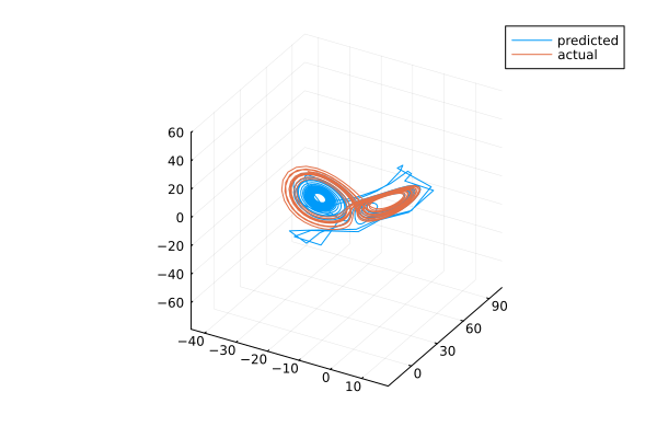
plot(transpose(output)[:, 1], transpose(output)[:, 2], transpose(output)[:, 3];
    label="predicted")
plot!(transpose(test)[:, 1], transpose(test)[:, 2], transpose(test)[:, 3];
    label="actual")