Continuous-Time Reservoirs from a SciMLProblem

ReservoirComputing.jl exposes a continuous-time reservoir layer, SciMLProblemReservoir, that wraps any AbstractSciMLProblem (ODEProblem, SDEProblem, DDEProblem) and plugs it into the standard collectstates / predict pipeline. The implementation lives in the RCODEReservoirExt package extension, so the extension is loaded automatically once SciMLBase and DataInterpolations are in scope. The user picks a concrete solver package (e.g. OrdinaryDiffEqTsit5, OrdinaryDiffEq) separately — its solver types are what the reservoir's args[1] consumes.

This page walks through the core type, how time is laid out internally, and a worked example that checks the continuous reservoir against a closed-form analytic solution.

Loading the extension

using ReservoirComputing
using LuxCore: setup
using SciMLBase
using DataInterpolations
using OrdinaryDiffEqTsit5    # or `OrdinaryDiffEq`, or whichever solver pkg you need

SciMLBase provides solve / remake, DataInterpolations is used for the per-window input signal in the autoregressive predict path, and the chosen OrdinaryDiffEq solver package brings the concrete solver type (Tsit5(), Euler(), …).

Constructing a reservoir from an ODE problem

The constructor follows the DiffEqFlux NeuralODE pattern:

SciMLProblemReservoir(prob, sampler, tspan, args...; kwargs...)

• prob — any AbstractSciMLProblem. The reservoir's initial state is taken from prob.u0; the ODE right-hand side reads the time-varying input through p.input(t) (injected by the extension at solve time).
• sampler — an AbstractSampler. The bundled TerminalStateSampling records the reservoir state at the end of each input window.
• tspan — overrides prob.tspan via remake at solve time. The input column grid is synthesised from tspan and the input width.
• args... — forwarded to solve positionally; the solver algorithm is the first element (Tsit5(), Euler(), …).
• kwargs... — forwarded to solve. The three keys saveat, save_everystep, and dense are owned by the helper and rejected at construction.

The user's ODE can carry static parameters as a NamedTuple (or nothing / NullParameters() if there are none). Anything else is rejected with an ArgumentError. The reserved name :input cannot appear in prob.p because the extension uses it to inject the interpolated input signal.

How time is laid out

collectstates receives a discrete data::AbstractMatrix of shape (channels, n_samples) and turns it into a continuous-time input:

1. tspan is split into n_samples equal-width windows of width Δt = (t1 - t0) / n_samples.
2. Input column k is held over window k (t0 + (k-1)Δt ≤ t < t0 + kΔt) via zero-order hold.
3. The reservoir state at the end of window k (t = t0 + kΔt) is sampled and becomes states[:, k].

This input-at-start / sample-at-end alignment matches the discrete update semantics: states[:, k] is the reservoir state after processing input k, with no off-by-one offset.

A worked example: linear ODE with closed-form solution

The scalar linear ODE dx/dt = -x + u(t) with u(t) = 1 and x(0) = 0 has the closed form x(t) = 1 - exp(-t). Running it through the continuous reservoir at a tight solver tolerance recovers that curve to within ~1e-6:

using ReservoirComputing
using LuxCore: setup
using SciMLBase
using DataInterpolations
using OrdinaryDiffEqTsit5
using Random

function linear_rhs!(dx, x, p, t)
    input_t = p.input(t)
    dx .= .-x .+ input_t
end

n_samples = 10
tspan = (0.0, 1.0)
Δt = (tspan[2] - tspan[1]) / n_samples
sample_ts = collect(range(tspan[1] + Δt, tspan[2]; length = n_samples))

u_const = 1.0
data = fill(u_const, 1, n_samples)
initial_state = [0.0]

prob = ODEProblem(linear_rhs!, initial_state, tspan, (;))
res = SciMLProblemReservoir(
    prob, TerminalStateSampling(), tspan, Tsit5();
    reltol = 1.0e-10, abstol = 1.0e-12
)
rc = ReservoirComputer(res, LinearReadout(1 => 1))
ps, st = setup(MersenneTwister(0), rc)

states, _ = collectstates(rc, data, ps, st)
analytic = u_const .* (1 .- exp.(.-sample_ts))

@assert states[1, :] ≈ analytic atol = 1.0e-6

Calling predict

Both predict signatures route through the same continuous helper:

predict(rc, data, ps, st)                  # teacher-forced
predict(rc, steps, ps, st; initialdata)    # autoregressive rollout

• The teacher-forced path solves the full tspan once and applies the readout column-by-column to the sampled states.
• The autoregressive path splits tspan into steps sub-intervals, feeds the previous readout output back as the constant input on the next sub-interval, and stitches the per-window readouts into the returned output matrix.

After train, pass the same st into predict so the rollout continues from the trained reservoir state. A fresh st starts from prob.u0.

Eye test: Lorenz chaos forecasting with a continuous ESN

The README example trains a discrete ESN on the Lorenz attractor and rolls it forward autoregressively. The same pipeline runs verbatim with SciMLProblemReservoir once you wrap the leaky-integrator continuous ESN equations

\[\frac{dx}{dt} = -x + \tanh\!\left(W_r\, x + W_{in}\, u(t) + b\right)\]

as an ODEProblem. The reservoir matrices are random, the readout is linear, and the only training step fits the linear readout on the collected continuous states.

using ReservoirComputing
using LuxCore: setup
using SciMLBase
using DataInterpolations
using OrdinaryDiffEqTsit5
using Plots
using Plots.PlotMeasures
using Random

Random.seed!(42)
rng = MersenneTwister(17)

# 1. Lorenz data
function lorenz!(du, u, p, t)
    du[1] = p[1] * (u[2] - u[1])
    du[2] = u[1] * (p[2] - u[3]) - u[2]
    du[3] = u[1] * u[2] - p[3] * u[3]
end
data_prob = ODEProblem(lorenz!, [1.0, 0.0, 0.0], (0.0, 40.0), [10.0, 28.0, 8 / 3])
data = Array(solve(data_prob, Tsit5(); saveat = 0.02))

shift, train_len, predict_len = 300, 1000, 250
input_data = data[:, shift:(shift + train_len - 1)]
target_data = data[:, (shift + 1):(shift + train_len)]
test = data[:, (shift + train_len):(shift + train_len + predict_len - 1)]

# 2. Continuous ESN reservoir parameters
N_res = 300
Wr = rand_sparse(rng, Float64, N_res, N_res; radius = 0.9, sparsity = 6 / N_res)
Win = scaled_rand(rng, Float64, N_res, 3)
bias = zeros(N_res)
initial_state = zeros(N_res)

# 3. Raw ODE equations — leaky-integrator continuous ESN
function ctesn_rhs!(dx, x, p, t)
    input_t = p.input(t)
    return dx .= .-x .+ tanh.(p.Wr * x .+ p.Win * input_t .+ p.b)
end

# 4. Wrap as SciMLProblemReservoir with Δt = 1 per input window
function build_rc(tspan_len)
    prob = ODEProblem(
        ctesn_rhs!, initial_state,
        (0.0, Float64(tspan_len)), (Wr = Wr, Win = Win, b = bias)
    )
    res = SciMLProblemReservoir(
        prob, TerminalStateSampling(),
        (0.0, Float64(tspan_len)), Tsit5();
        reltol = 1.0e-6, abstol = 1.0e-8
    )
    return ReservoirComputer(res, (NLAT2(),), LinearReadout(N_res => 3))
end

rc_train = build_rc(train_len)
rc_predict = build_rc(predict_len)
ps, st = setup(rng, rc_train)

# 5. Fit the linear readout on the collected continuous states
ps, st = train(rc_train, input_data, target_data, ps, st;
    objective = RidgeRegression(1.0e-6))

# 6. Autoregressive rollout under the same continuous dynamics
output, _ = predict(rc_predict, predict_len, ps, st; initialdata = test[:, 1])

dt = 0.02
lorenz_maxlyap = 0.9056
lyap_time = (0:(predict_len - 1)) .* dt .* (1 / lorenz_maxlyap)

p1 = plot(lyap_time, [test[1, :] output[1, :]]; label = ["actual" "predicted"],
    ylabel = "x(t)", linewidth = 2.5, xticks = false, yticks = -15:15:15);
p2 = plot(lyap_time, [test[2, :] output[2, :]]; label = ["actual" "predicted"],
    ylabel = "y(t)", linewidth = 2.5, xticks = false, yticks = -20:20:20);
p3 = plot(lyap_time, [test[3, :] output[3, :]]; label = ["actual" "predicted"],
    ylabel = "z(t)", linewidth = 2.5, xlabel = "max(λ)*t", yticks = 10:15:40);

plot(p1, p2, p3; plot_title = "Lorenz System Coordinates",
    layout = (3, 1), xtickfontsize = 12, ytickfontsize = 12, xguidefontsize = 15,
    yguidefontsize = 15,
    legendfontsize = 12, titlefontsize = 20)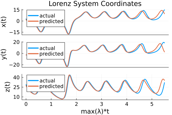

The two trajectories should agree on the early portion of the rollout before chaotic divergence — exactly the behaviour the discrete-ESN example produces. The point of the eye test is that nothing in the training loop changes: train and predict still drive the SciMLProblemReservoir through the same pipeline they use for any discrete reservoir.

A delay-equation target: Mackey-Glass

SciMLProblemReservoir wraps anyAbstractSciMLProblem, so the training data — and, if you want, the reservoir itself — can come from a delay-differential equation, a stochastic equation, or any other SciML problem type. The smallest non-trivial demonstration: forecast the Mackey-Glass time series, a 1-D delay equation that has been a reservoir-computing benchmark for two decades.

using ReservoirComputing
using LuxCore: setup
using SciMLBase
using DataInterpolations
using OrdinaryDiffEqTsit5
using LinearAlgebra
using Plots
using Random
using Statistics

Random.seed!(42)
rng = MersenneTwister(17)

# Mackey-Glass: dx/dt = β x(t-τ) / (1 + x(t-τ)^n) - γ x(t).
# With τ = 17 the trajectory is chaotic.
const β_mg, γ_mg, n_mg, τ_mg = 0.2, 0.1, 10, 17.0
function mackey_glass!(dx, x, h, p, t)
    x_delay = h(p, t - τ_mg)[1]
    return dx[1] = β_mg * x_delay / (1 + x_delay^n_mg) - γ_mg * x[1]
end
mg_history(p, t) = [1.2]

mg_data_prob = DDEProblem(mackey_glass!, [1.2], mg_history, (0.0, 1500.0);
    constant_lags = [τ_mg])

# Use a fixed-step recurrence so this documentation example remains independent
# of a particular delay-solver implementation.
mg_data = zeros(1, 1501)
mg_data[1, 1] = 1.2
for step in 1:1500
    x = mg_data[1, step]
    x_delay = step > Int(τ_mg) ? mg_data[1, step - Int(τ_mg)] : 1.2
    mg_data[1, step + 1] = x + β_mg * x_delay / (1 + x_delay^n_mg) - γ_mg * x
end

shift, train_len, predict_len = 200, 1000, 200
input_data = mg_data[:, shift:(shift + train_len - 1)]
target_data = mg_data[:, (shift + 1):(shift + train_len)]
test_data = mg_data[:, (shift + train_len):(shift + train_len + predict_len - 1)]

# Same continuous ESN reservoir machinery as the Lorenz example, retuned
# for the much smaller Mackey-Glass amplitude (~1, vs Lorenz ~20).
N_res = 150
sparsity = 6 / N_res
Wr_raw = randn(rng, N_res, N_res) .* (rand(rng, N_res, N_res) .< sparsity)
Wr = (0.9 / maximum(abs.(eigvals(Wr_raw)))) .* Wr_raw
Win = 0.05 .* randn(rng, N_res, 1)
bias = 0.0 .* randn(rng, N_res)
initial_state = zeros(N_res)

function mg_reservoir_rhs!(dx, x, p, t)
    input_t = p.input(t)
    return dx .= .-x .+ tanh.(p.Wr * x .+ p.Win * input_t .+ p.b)
end

function build_mg_rc(n_steps)
    tspan = (0.0, n_steps * 1.0)
    prob = ODEProblem(mg_reservoir_rhs!, initial_state, tspan,
        (Wr = Wr, Win = Win, b = bias))
    res = SciMLProblemReservoir(prob, TerminalStateSampling(), tspan, Tsit5();
        reltol = 1.0e-6, abstol = 1.0e-8)
    return ReservoirComputer(res, (NLAT2(),), LinearReadout(N_res => 1))
end

rc_mg_train = build_mg_rc(train_len)
rc_mg_predict = build_mg_rc(predict_len)
ps_mg, st_mg = setup(rng, rc_mg_train)
ps_mg, st_mg = train(rc_mg_train, input_data, target_data, ps_mg, st_mg;
    objective = RidgeRegression(1.0e-6), washout = 0)

mg_output, _ = predict(rc_mg_predict, predict_len, ps_mg, st_mg;
    initialdata = test_data[:, 1])

plot([test_data[1, :], mg_output[1, :]];
    label = ["actual" "predicted"], linewidth = 2,
    xlabel = "step", ylabel = "x(t)",
    title = "Mackey-Glass (τ=17) — continuous ESN rollout")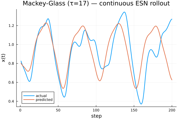

Two things to notice:

• The data path constructs the corresponding DDEProblem and uses a fixed-step recurrence to keep this documentation example deterministic. The reservoir wrapper only cares about the resulting matrix shape, so production code can instead solve mg_data_prob with a compatible delay solver.
• The reservoir is kept as an ODEProblem for simplicity. Because SciMLProblemReservoir's prob field is untyped, it would equally accept a DDEProblem of the form dx/dt = -x(t) + tanh(W_r x(t-τ_r) + W_{in} u(t) + b) — useful when the target has long-range temporal correlations. Delay-coupled reservoirs of that form are explored in the CTESN/delay-reservoir literature; a tuned implementation will land in PR3.

As with the Lorenz example, this is a demonstration of the new plumbing rather than an optimised benchmark: hyperparameters were tuned by hand to land a watchable forecast, not chosen via cross-validation.

Adding your own sampler

The reservoir state sequence the readout sees is produced by an AbstractSampler. To plug in a custom strategy (window mean, sub-sampling within a window, etc.), define a concrete subtype and a matching __sample(::YourSampler, sol) method inside an extension that also loads OrdinaryDiffEq and SciMLBase. The method should return a (state_dim, n_samples) matrix; everything downstream (state modifiers, readout, predict) is sampler-agnostic.