Callback Library
DiffEqCallbacks.jl provides a library of various helpful callbacks which can be used with any component solver which implements the callback interface. It adds the following callbacks which are available to users of DifferentialEquations.jl.
Manifold Conservation and Projection
In many cases, you may want to declare a manifold on which a solution lives. Mathematically, a manifold M is defined by a function g as the set of points where g(u)=0. An embedded manifold can be a lower dimensional object which constrains the solution. For example, g(u)=E(u)-C where E is the energy of the system in state u, meaning that the energy must be constant (energy preservation). Thus by defining the manifold the solution should live on, you can retain desired properties of the solution.
It is a consequence of convergence proofs both in the deterministic and stochastic cases that post-step projection to manifolds keep the same convergence rate (stochastic requires a truncation in the proof, details details), thus any algorithm can be easily extended to conserve properties. If the solution is supposed to live on a specific manifold or conserve such property, this guarantees the conservation law without modifying the convergence properties.
Constructor
ManifoldProjection(g; nlsolve=NLSOLVEJL_SETUP(), save=true, autonomous=numargs(g)==2, nlopts=Dict{Symbol,Any}())g: The residual function for the manifold. This is an inplace function of formg(u, resid)org(t, u, resid)which writes to the residual the difference from the manifold components.nlsolve: A nonlinear solver as defined in the nlsolve format.save: Whether to do the standard saving (applied after the callback).autonomous: Whethergis an autonomous function of the formg(u, resid).nlopts: Optional arguments to nonlinear solver which can be any of the NLsolve keywords.
Example
Here we solve the harmonic oscillator:
u0 = ones(2)
function f(t,u,du)
  du[1] = u[2]
  du[2] = -u[1]
end
prob = ODEProblem(f,u0,(0.0,100.0))
However, this problem is supposed to conserve energy, and thus we define our manifold to conserve the sum of squares:
function g(u,resid)
  resid[1] = u[2]^2 + u[1]^2 - 2
  resid[2] = 0
end
To build the callback, we just call
cb = ManifoldProjection(g)Using this callback, the Runge-Kutta method Vern7 conserves energy:
sol = solve(prob,Vern7(),callback=cb)
@test sol[end][1]^2 + sol[end][2]^2 ≈ 2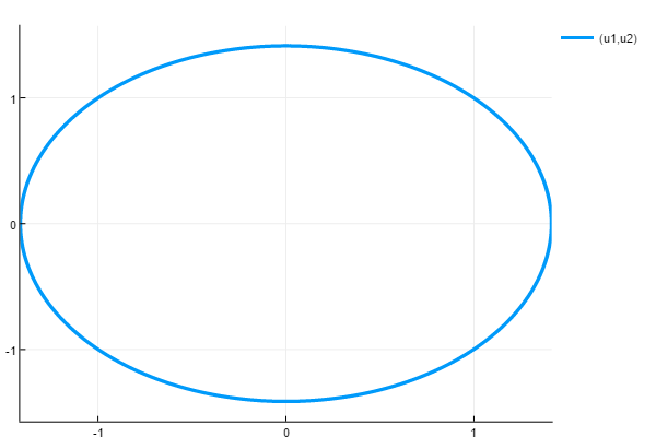
AutoAbstol
Many problem solving environments such as MATLAB provide a way to automatically adapt the absolute tolerance to the problem. This helps the solvers automatically "learn" what appropriate limits are. Via the callback interface, DiffEqCallbacks.jl implements a callback AutoAbstol which has the same behavior as the MATLAB implementation, that is the absolute tolerance starts and at each iteration it is set to the maximum value that the state has thus far reached times the relative tolerance. If init_curmax is zero, then the initial value is determined by the abstol of the solver. Otherwise this is the initial value for the current maximum abstol.
To generate the callback, use the constructor:
AutoAbstol(save=true;init_curmax=0.0)PositiveDomain
Especially in biology and other natural sciences, a desired property of dynamical systems is the positive invariance of the positive cone, i.e. non-negativity of variables at time $t_0$ ensures their non-negativity at times $t \geq t_0$ for which the solution is defined. However, even if a system satisfies this property mathematically it can be difficult for ODE solvers to ensure it numerically, as these MATLAB examples show.
In order to deal with this problem one can specify isoutofdomain=(t,u) -> any(x -> x < 0, u) as additional solver option, which will reject any step that leads to non-negative values and reduce the next time step. However, since this approach only rejects steps and hence calculations might be repeated multiple times until a step is accepted, it can be computationally expensive.
Another approach is taken by a PositiveDomain callback in DiffEqCallbacks.jl, which is inspired by Shampine's et al. paper about non-negative ODE solutions. It reduces the next step by a certain scale factor until the extrapolated value at the next time point is non-negative with a certain tolerance. Extrapolations are cheap to compute but might be inaccurate, so if a time step is changed it is additionally reduced by a safety factor of 0.9. Since extrapolated values are only non-negative up to a certain tolerance and in addition actual calculations might lead to negative values, also any negative values at the current time point are set to 0. Hence by this callback non-negative values at any time point are ensured in a computationally cheap way, but the quality of the solution depends on how accurately extrapolations approximate next time steps.
Please note that the system should be defined also outside the positive domain, since even with these approaches negative variables might occur during the calculations. Moreover, one should follow Shampine's et. al. advice and set the derivative $x'_i$ of a negative component $x_i$ to $\max \{0, f_i(t, x)\}$, where $t$ denotes the current time point with state vector $x$ and $f_i$ is the $i$-th component of function $f$ in an ODE system $x' = f(t, x)$.
Constructor
PositiveDomain(u=nothing; save=true, abstol=nothing, scalefactor=nothing)u: A prototype of the state vector of the integrator. A copy of it is saved and extrapolated values are written to it. If it is not specified every application of the callback allocates a new copy of the state vector.save: Whether to do the standard saving (applied after the callback).abstol: Tolerance up to which negative extrapolated values are accepted. Element-wise tolerances are allowed. If it is not specified every application of the callback uses the current absolute tolerances of the integrator.scalefactor: Factor by which an unaccepted time step is reduced. If it is not specified time steps are halved.
GeneralDomain
A GeneralDomain callback in DiffEqCallbacks.jl generalizes the concept of a PositiveDomain callback to arbitrary domains. Domains are specified by in-place functions g(u, resid) or g(t, u, resid) that calculate residuals of a state vector u at time t relative to that domain. As for PositiveDomain, steps are accepted if residuals of the extrapolated values at the next time step are below a certain tolerance. Moreover, this callback is automatically coupled with a ManifoldProjection that keeps all calculated state vectors close to the desired domain, but in contrast to a PositiveDomain callback the nonlinear solver in a ManifoldProjection can not guarantee that all state vectors of the solution are actually inside the domain. Thus a PositiveDomain callback should in general be preferred.
Constructor
function GeneralDomain(g, u=nothing; nlsolve=NLSOLVEJL_SETUP(), save=true,
                       abstol=nothing, scalefactor=nothing, autonomous=numargs(g)==2,
nlopts=Dict(:ftol => 10*eps()))g: The residual function for the domain. This is an inplace function of formg(u, resid)org(t, u, resid)which writes to the residual the difference from the domain.u: A prototype of the state vector of the integrator and the residuals. Two copies of it are saved, and extrapolated values and residuals are written to them. If it is not specified every application of the callback allocates two new copies of the state vector.nlsolve: A nonlinear solver as defined in the nlsolve format which is passed to aManifoldProjection.save: Whether to do the standard saving (applied after the callback).abstol: Tolerance up to which residuals are accepted. Element-wise tolerances are allowed. If it is not specified every application of the callback uses the current absolute tolerances of the integrator.scalefactor: Factor by which an unaccepted time step is reduced. If it is not specified time steps are halved.autonomous: Whethergis an autonomous function of the formg(u, resid).nlopts: Optional arguments to nonlinear solver of aManifoldProjectionwhich can be any of the NLsolve keywords. The default value offtol = 10*eps()ensures that convergence is only declared if the infinite norm of residuals is very small and hence the state vector is very close to the domain.
Stepsize Limiters
In many cases there is a known maximal stepsize for which the computation is stable and produces correct results. For example, in hyperbolic PDEs one normally needs to ensure that the stepsize stays below some $\Delta t_{FE}$ determined by the CFL condition. For nonlinear hyperbolic PDEs this limit can be a function dtFE(t,u) which changes throughout the computation. The stepsize limiter lets you pass a function which will adaptively limit the stepsizes to match these constraints.
Constructor
StepsizeLimiter(dtFE;safety_factor=9//10,max_step=false,cached_dtcache=0.0)dtFE: The function for the maximal timestep. Calculated using the previoustandu.safety_factor: The factor below the true maximum that will be stepped to which defaults to9//10.max_step: Makes every step equal tosafety_factor*dtFE(t,u)when the solver is set toadaptive=false.cached_dtcache: Should be set to match the type for time when not using Float64 values.
SavingCallback
The saving callback lets you define a function save_func(t, u, integrator) which returns quantities of interest that shall be saved.
Constructor
SavingCallback(save_func, saved_values::SavedValues;
               saveat=Vector{eltype(saved_values.t)}(),
               save_everystep=isempty(saveat),
               tdir=1)
save_func(t, u, integrator)returns the quantities which shall be saved.saved_values::SavedValuescontains vectorst::Vector{tType},saveval::Vector{savevalType}of the saved quantities. Here,save_func(t, u, integrator)::savevalType.saveatMimickssaveatinsolvefor ODEs.save_everystepMimickssave_everystepinsolvefor ODEs.tdirshould besign(tspan[end]-tspan[1]). It defaults to1and should be adapted iftspan[1] > tspan[end].
IterativeCallback
IterativeCallback is a callback to be used to iteratively apply some affect. For example, if given the first effect at t₁, you can define t₂ to apply the next effect.
A IterativeCallback is constructed as follows:
function IterativeCallback(time_choice, user_affect!,tType = Float64;
                           initialize = DiffEqBase.INITIALIZE_DEFAULT,
                           initial_affect = false, kwargs...)
where time_choice(integrator) determines the time of the next callback and user_affect! is the effect applied to the integrator at the stopping points.
PeriodicCallback
PeriodicCallback can be used when a function should be called periodically in terms of integration time (as opposed to wall time), i.e. at t = tspan[1], t = tspan[1] + Δt, t = tspan[1] + 2Δt, and so on. This callback can, for example, be used to model a digital controller for an analog system, running at a fixed rate.
Constructor
PeriodicCallback(f, Δt::Number; kwargs...)where f is the function to be called periodically, Δt is the period, and kwargs are keyword arguments accepted by the DiscreteCallback constructor (see the DiscreteCallback section).