Stochastic Differential Equations

This tutorial will introduce you to the functionality for solving SDEs. Other introductions can be found by checking out DiffEqTutorials.jl. This tutorial assumes you have read the Ordinary Differential Equations tutorial.

Example 1: Scalar SDEs

In this example we will solve the equation

where $f(t,u)=αu$ and $g(t,u)=βu$. We know via Stochastic Calculus that the solution to this equation is

To solve this numerically, we define a problem type by giving it the equation and the initial condition:

using DifferentialEquations
α=1
β=1
u₀=1/2
f(t,u) = α*u
g(t,u) = β*u
dt = 1//2^(4)
tspan = (0.0,1.0)
prob = SDEProblem(f,g,u₀,(0.0,1.0))

The solve interface is then the same as with ODEs. Here we will use the classic Euler-Maruyama algorithm EM and plot the solution:

sol = solve(prob,EM(),dt=dt)
using Plots; plotly() # Using the Plotly backend
plot(sol)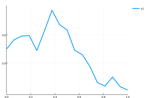

Using Higher Order Methods

One unique feature of DifferentialEquations.jl is that higher-order methods for stochastic differential equations are included. For reference, let's also give the SDEProblem the analytical solution. We can do this by making a test problem. This can be a good way to judge how accurate the algorithms are, or is used to test convergence of the algorithms for methods developers. Thus we define the problem object with:

f(::Type{Val{:analytic}},t,u₀,W) = u₀*exp((α-(β^2)/2)*t+β*W)
prob = SDEProblem(f,g,u₀,(0.0,1.0))

and then we pass this information to the solver and plot:

#We can plot using the classic Euler-Maruyama algorithm as follows:
sol = solve(prob,EM(),dt=dt)
plot(sol,plot_analytic=true)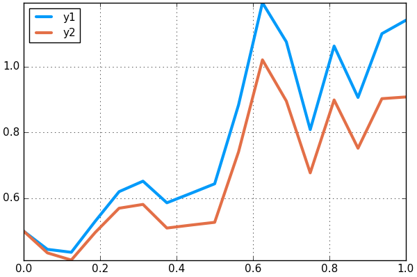

We can choose a higher-order solver for a more accurate result:

sol = solve(prob,SRIW1(),dt=dt,adaptive=false)
plot(sol,plot_analytic=true)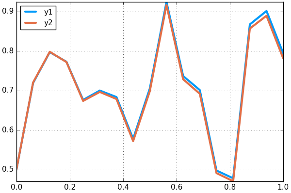

By default, the higher order methods have adaptivity. Thus one can use

sol = solve(prob,SRIW1())
plot(sol,plot_analytic=true)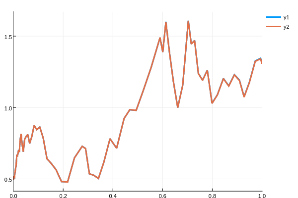

Here we allowed the solver to automatically determine a starting dt. This estimate at the beginning is conservative (small) to ensure accuracy. We can instead start the method with a larger dt by passing in a value for the starting dt:

sol = solve(prob,SRIW1(),dt=dt)
plot(sol,plot_analytic=true)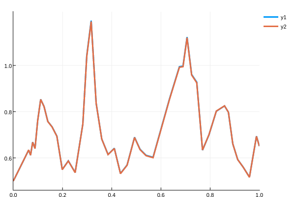

Monte Carlo Simulations

Instead of solving single trajectories, we can turn our problem into a MonteCarloProblem to solve many trajectories all at once. This is done by the MonteCarloProblem constructor:

monte_prob = MonteCarloProblem(prob)

The solver commands are defined at the Monte Carlo page. For example we can choose to have 1000 trajectories via num_monte=1000. In addition, this will automatically parallelize using Julia native parallelism if extra processes are added via addprocs(), but we can change this to use multithreading via parallel_type=:threads. Together, this looks like:

sol = solve(monte_prob,num_monte=1000,paralle_type=:threads)

Many more controls are defined at the Monte Carlo page, including analysis tools. A very simple analysis can be done with the MonteCarloSummary, which builds mean/var statistics and has an associated plot recipe. For example, we can get the statistics at every 0.01 timesteps and plot the average + error using:

summ = MonteCarloSummary(sol,0:0.01:1)
plot(summ,labels="Middle 95%")
summ = MonteCarloSummary(sol,0:0.01:1;quantiles=[0.25,0.75])
plot!(summ,labels="Middle 50%",legend=true)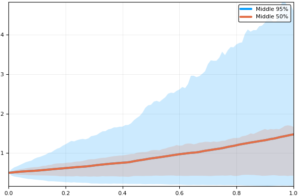

Additionally we can easily calculate the correlation between the values at t=0.2 and t=0.7 via

timepoint_meancor(sim,0.2,0.7) # Gives both means and then the correlation coefficient

Example 2: Systems of SDEs with Diagonal Noise

Generalizing to systems of equations is done in the same way as ODEs. In this case, we can define both f and g as in-place functions. Without any other input, the problem is assumed to have diagonal noise, meaning that each component of the system has a unique Wiener process. Thus f(t,u,du) gives a vector of du which is the deterministic change, and g(t,u,du2) gives a vector du2 for which du2.*W is the stochastic portion of the equation.

For example, the Lorenz equation with additive noise has the same deterministic portion as the Lorenz equations, but adds an additive noise, which is simply 3*N(0,dt) where N is the normal distribution dt is the time step, to each step of the equation. This is done via:

function lorenz(t,u,du)
  du[1] = 10.0(u[2]-u[1])
  du[2] = u[1]*(28.0-u[3]) - u[2]
  du[3] = u[1]*u[2] - (8/3)*u[3]
end

function σ_lorenz(t,u,du)
  du[1] = 3.0
  du[2] = 3.0
  du[3] = 3.0
end

prob_sde_lorenz = SDEProblem(lorenz,σ_lorenz,[1.0,0.0,0.0],(0.0,10.0))
sol = solve(prob_sde_lorenz)
plot(sol,vars=(1,2,3))

Note that it's okay for the noise function to mix terms. For example

function σ_lorenz(t,u,du)
  du[1] = sin(u[3])*3.0
  du[2] = u[2]*u[1]*3.0
  du[3] = 3.0
end

is a valid noise function, which will once again give diagonal noise by du2.*W. Note also that in this format, it is fine to use ParameterizedFunctions. For example, the Lorenz equation could have been defined as:

f = @ode_def_nohes LorenzSDE begin
  dx = σ*(y-x)
  dy = x*(ρ-z) - y
  dz = x*y - β*z
end σ=>10. ρ=>28. β=>2.66

g = @ode_def_nohes LorenzSDENoise begin
  dx = α
  dy = α
  dz = α
end α=>3.0

Example 3: Systems of SDEs with Scalar Noise

In this example we'll solve a system of SDEs with scalar noise. This means that the same noise process is applied to all SDEs. First we need to define a scalar noise process using the Noise Process interface. Since we want a WienerProcess that starts at 0.0 at time 0.0, we use the command W = WienerProcess(0.0,0.0,0.0) to define the Brownian motion we want, and then give this to the noise option in the SDEProblem. For a full example, let's solve a linear SDE with scalar noise using a high order algorithm:

f(t,u,du) = (du .= u)
g(t,u,du) = (du .= u)
u0 = rand(4,2)

W = WienerProcess(0.0,0.0,0.0)
prob = SDEProblem(f,g,u0,(0.0,1.0),noise=W)
sol = solve(prob,SRIW1())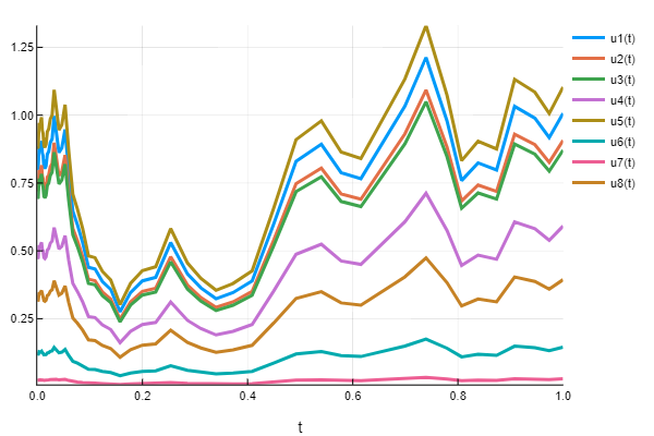

Example 4: Systems of SDEs with Non-Diagonal Noise

In the previous examples we had diagonal noise, that is a vector of random numbers dW whose size matches the output of g where the noise is applied element-wise, and scalar noise where a single random variable is applied to all dependent variables. However, a more general type of noise allows for the terms to linearly mixed (note that nonlinear mixings are not SDEs but fall under the more general class of random ordinary differential equations (RODEs) which have a separate set of solvers.

Let's define a problem with four Wiener processes and two dependent random variables. In this case, we will want the output of g to be a 2x4 matrix, such that the solution is g(t,u)*dW, the matrix multiplication. For example, we can do the following:

f(t,u,du) = du .= 1.01u
function g(t,u,du)
  du[1,1] = 0.3u[1]
  du[1,2] = 0.6u[1]
  du[1,3] = 0.9u[1]
  du[1,4] = 0.12u[2]
  du[2,1] = 1.2u[1]
  du[2,2] = 0.2u[2]
  du[2,3] = 0.3u[2]
  du[2,4] = 1.8u[2]
end
prob = SDEProblem(f,g,ones(2),(0.0,1.0),noise_rate_prototype=zeros(2,4))

In our g we define the functions for computing the values of the matrix. The matrix itself is determined by the keyword argument noise_rate_prototype in the SDEProblem constructor. This is a prototype for the type that du will be in g. This can be any AbstractMatrix type. Thus for example, we can define the problem as

# Define a sparse matrix by making a dense matrix and setting some values as not zero
A = zeros(2,4)
A[1,1] = 1
A[1,4] = 1
A[2,4] = 1
sparse(A)

# Make `g` write the sparse matrix values
function g(t,u,du)
  du[1,1] = 0.3u[1]
  du[1,4] = 0.12u[2]
  du[2,4] = 1.8u[2]
end

# Make `g` use the sparse matrix
prob = SDEProblem(f,g,ones(2),(0.0,1.0),noise_rate_prototype=A)

and now g(t,u) writes into a sparse matrix, and g(t,u)*dW is sparse matrix multiplication.

Example 4: Colored Noise

Colored noise can be defined using the Noise Process interface. In that portion of the docs, it is shown how to define your own noise process my_noise, which can be passed to the SDEProblem

SDEProblem(f,g,u0,tspan,noise=my_noise)

Example: Spatially-Colored Noise in the Heston Model

Let's define the Heston equation from financial mathematics:

In this problem, we have a diagonal noise problem given by:

function f(t,u,du)
  du[1] = μ*u[1]
  du[2] = κ*(Θ-u[2])
end
function g(t,u,du)
  du[1] = √u[2]*u[1]
  du[2] = Θ*√u[2]
end

However, our noise has a correlation matrix for some constant ρ. Choosing ρ=0.2:

Γ = [1 ρ;ρ 1]

To solve this, we can define a CorrelatedWienerProcess which starts at zero (W(0)=0) via:

heston_noise = CorrelatedWienerProcess!(Γ,tspan[1],zeros(2),zeros(2))

This is then used to build the SDE:

SDEProblem(f,g,u0,tspan,noise=heston_noise)

Of course, to fully define this problem we need to define our constants. Constructors for making common models like this easier to define can be found in the modeling toolkits. For example, the HestonProblem is pre-defined as part of the financial modeling tools.