Bayesian Physics informed Neural Network ODEs Solvers

Bayesian inference for PINNs provides an approach to ODE solution finding and parameter estimation with quantified uncertainty.

using ModelingToolkit, NeuralPDE, SciMLBase, AdvancedHMC, MCMCChains, LogDensityProblems

The Lotka-Volterra Model

The Lotka–Volterra equations, also known as the predator–prey equations, are a pair of first-order nonlinear differential equations. These differential equations are frequently used to describe the dynamics of biological systems in which two species interact, one as a predator and the other as prey. The populations change through time according to the pair of equations:

\[\begin{aligned} \frac{\mathrm{d}x}{\mathrm{d}t} &= (\alpha - \beta y(t))x(t), \\ \frac{\mathrm{d}y}{\mathrm{d}t} &= (\delta x(t) - \gamma)y(t) \end{aligned}\]

where $x(t)$ and $y(t)$ denote the populations of prey and predator at time $t$, respectively, and $\alpha, \beta, \gamma, \delta$ are positive parameters.

We implement the Lotka-Volterra model and simulate it with ideal parameters $\alpha = 1.5$, $\beta = 1$, $\gamma = 3$, and $\delta = 1$ and initial conditions $x(0) = y(0) = 1$.

We then solve the equations and estimate the parameters of the model with priors for $\alpha$, $\beta$, $\gamma$ and $\delta$ as Normal(1,2), Normal(2,2), Normal(2,2) and Normal(0,2) using a neural network.

using ModelingToolkit, NeuralPDE, SciMLBase, AdvancedHMC, MCMCChains, LogDensityProblems,
    Lux, Plots, OrdinaryDiffEq, Distributions, Random

function lotka_volterra(u, p, t)
    # Model parameters.
    α, β, γ, δ = p
    # Current state.
    x, y = u

    # Evaluate differential equations.
    dx = (α - β * y) * x # prey
    dy = (δ * x - γ) * y # predator

    return [dx, dy]
end

# initial-value problem.
u0 = [1.0, 1.0]
p = [1.5, 1.0, 3.0, 1.0]
tspan = (0.0, 4.0)
prob = ODEProblem(lotka_volterra, u0, tspan, p)

ODEProblem with uType Vector{Float64} and tType Float64. In-place: false
Non-trivial mass matrix: false
timespan: (0.0, 4.0)
u0: 2-element Vector{Float64}:
 1.0
 1.0

With the saveat argument, we can specify that the solution is stored only at saveat time units.

# Solve using OrdinaryDiffEq.jl solver
dt = 0.01
solution = solve(prob, Tsit5(); saveat = dt)

retcode: Success
Interpolation: 1st order linear
t: 401-element Vector{Float64}:
 0.0
 0.01
 0.02
 0.03
 0.04
 0.05
 0.06
 0.07
 0.08
 0.09
 ⋮
 3.92
 3.93
 3.94
 3.95
 3.96
 3.97
 3.98
 3.99
 4.0
u: 401-element Vector{Vector{Float64}}:
 [1.0, 1.0]
 [1.0051122697054304, 0.9802235489841001]
 [1.0104482482084793, 0.9608884029133249]
 [1.0160067852516195, 0.9419859539931972]
 [1.0217868581271055, 0.9235077034160883]
 [1.0277875716769742, 0.9054452613612181]
 [1.0340081582930438, 0.887790346994655]
 [1.040447977916915, 0.870534788469315]
 [1.0471065141055134, 0.8536705240234226]
 [1.0539833005834183, 0.837189627503347]
 ⋮
 [1.7188602790655703, 0.35603128520071003]
 [1.7386754231380195, 0.35153232204585927]
 [1.7587969344457686, 0.3471593575148184]
 [1.779227949981121, 0.34291022060855736]
 [1.7999716537968578, 0.3387828301940905]
 [1.821031277006269, 0.3347751950044705]
 [1.8424100977831226, 0.3308854136387941]
 [1.8641114413617017, 0.3271116745621956]
 [1.886138680036769, 0.32345225610585315]

We generate noisy observations to use for the parameter estimation task in this tutorial. To make the example more realistic we add random normally distributed noise to the simulation.

# Dataset creation for parameter estimation (30% noise)
time = solution.t
u = hcat(solution.u...)
x = u[1, :] + (u[1, :]) .* (0.3 .* randn(length(u[1, :])))
y = u[2, :] + (u[2, :]) .* (0.3 .* randn(length(u[2, :])))
dataset = [x, y, time]

# Plotting the data which will be used
plot(time, x, label = "noisy x")
plot!(time, y, label = "noisy y")
plot!(solution, labels = ["x" "y"])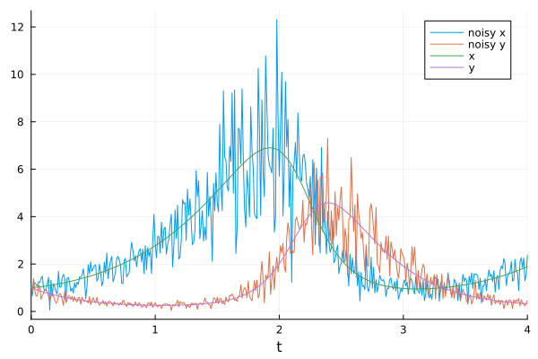

Let's define a PINN.

# Neural Networks must have 2 outputs as u -> [dx,dy] in function lotka_volterra()
chain = Chain(Dense(1, 6, tanh), Dense(6, 6, tanh), Dense(6, 2))

Chain(
    layer_1 = Dense(1 => 6, tanh),                # 12 parameters
    layer_2 = Dense(6 => 6, tanh),                # 42 parameters
    layer_3 = Dense(6 => 2),                      # 14 parameters
)         # Total: 68 parameters,
          #        plus 0 states.

The dataset we generated can be passed for doing parameter estimation using provided priors in param keyword argument for BNNODE.

alg = BNNODE(chain;
    dataset = dataset,
    draw_samples = 1000,
    l2std = [0.1, 0.1],
    phystd = [0.1, 0.1],
    priorsNNw = (0.0, 3.0),
    param = [
        Normal(1, 2),
        Normal(2, 2),
        Normal(2, 2),
        Normal(0, 2)], progress = false)

sol_pestim = solve(prob, alg; saveat = dt)

The solution for the ODE is returned as a nested vector sol_flux_pestim.ensemblesol. Here, [$x$ , $y$] would be returned.

# plotting solution for x,y for chain
plot(time, sol_pestim.ensemblesol[1], label = "estimated x")
plot!(time, sol_pestim.ensemblesol[2], label = "estimated y")

# comparing it with the original solution
plot!(solution, labels = ["true x" "true y"])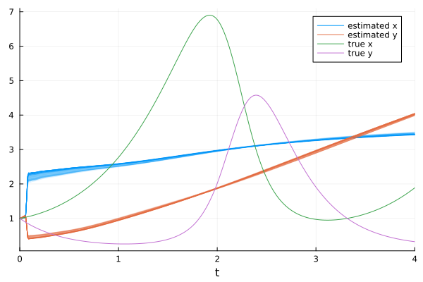

We can see the estimated ODE parameters by -

sol_pestim.estimated_de_params

4-element Vector{MonteCarloMeasurements.Particles{Float64, 334}}:
  0.162 ± 0.024
  0.0268 ± 0.0058
 -2.26 ± 0.24
 -0.579 ± 0.074

We can see it is close to the true values of the parameters.