Data Arrays

In many cases, a standard array may not be enough to fully hold the data for a model. Many of the solvers in DifferentialEquations.jl allow you to solve problems on AbstractArray types which allow you to extend the meaning of an array. The DEDataArray{T} type allows one to add other "non-continuous" variables to an array, which can be useful in many modeling situations involving lots of events.

The Data Array Interface

To define an DEDataArray, make a type which subtypes DEDataArray{T} with a field x for the "array of continuous variables" for which you would like the differential equation to treat directly. For example:

type MyDataArray{T} <: DEDataArray{T}
    x::Array{T,1}
    a::T
    b::Symbol
end

In this example, our resultant array is a SimType, and its data which is presented to the differential equation solver will be the array x. Any array which the differential equation solver can use is allowed to be made as the field x, including other DEDataArrays. Other than that, you can add whatever fields you please, and let them be whatever type you please. These extra fields are carried along in the differential equation solver that the user can use in their f equation and modify via callbacks.

Example: A Control Problem

In this example we will use a DEDataArray to solve a problem where control parameters change at various timepoints. First we will build

type SimType{T} <: DEDataArray{T}
    x::Array{T,1}
    f1::T
end

as our DEDataArray. It has an extra field f1 which we will use as our control variable. Our ODE function will use this field as follows:

function f(t,u,du)
    du[1] = -0.5*u[1] + u.f1
    du[2] = -0.5*u[2]
end

Now we will setup our control mechanism. It will be a simple setup which uses set timepoints at which we will change f1. At t=5.0 we will want to increase the value of f1, and at t=8.0 we will want to decrease the value of f1. Using the DiscreteCallback interface, we code these conditions as follows:

const tstop1 = [5.]
const tstop2 = [8.]


function condition(t,u,integrator)
  t in tstop1
end

function condition2(t,u,integrator)
  t in tstop2
end

Now we have to apply an affect when these conditions are reached. When condition is hit (at t=5.0), we will increase f1 to 1.5. When condition2 is reached, we will decrease f1 to -1.5. This is done via the affects:

function affect!(integrator)
  for c in user_cache(integrator)
    c.f1 = 1.5
  end
end

function affect2!(integrator)
  for c in user_cache(integrator)
    c.f1 = -1.5
  end
end

Notice that we have to loop through the user_cache array (provided by the integrator interface) to ensure that all internal caches are also updated. With these functions we can build our callbacks:

save_positions = (true,true)

cb = DiscreteCallback(condition, affect!, save_positions)

save_positions = (false,true)

cb2 = DiscreteCallback(condition2, affect2!, save_positions)

cbs = CallbackSet(cb,cb2)

Now we define our initial condition. We will start at [10.0;10.0] with f1=0.0.

u0 = SimType([10.0;10.0], 0.0)
prob = ODEProblem(f,u0,(0.0,10.0))

Lastly we solve the problem. Note that we must pass tstop values of 5.0 and 8.0 to ensure the solver hits those timepoints exactly:

const tstop = [5.;8.]
sol = solve(prob,Tsit5(),callback = cbs, tstops=tstop)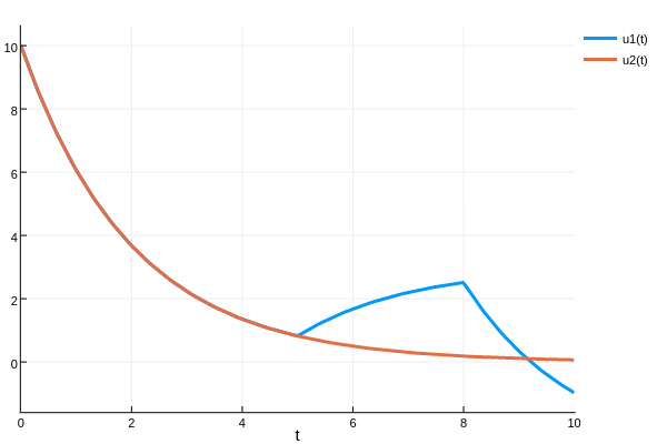

It's clear from the plot how the controls affected the outcome.

Data Arrays vs ParameterizedFunctions

The reason for using a DEDataArray is because the solution will then save the control parameters. For example, we can see what the control parameter was at every timepoint by checking:

[sol[i].f1 for i in 1:length(sol)]

A similar solution can be achieved using a ParameterizedFunction. We could have instead created our function as:

function f(t,u,param,du)
    du[1] = -0.5*u[1] + param
    du[2] = -0.5*u[2]
end
pf = ParameterizedFunction(f,0.0)
u0 = SimType([10.0;10.0], 0.0)
prob = ODEProblem(f,u0,(0.0,10.0))
const tstop = [5.;8.]
sol = solve(prob,Tsit5(),callback = cbs, tstops=tstop)

where we now change the callbacks to changing the parameter in the function:

function affect!(integrator)
  integrator.f.params = 1.5
end

function affect2!(integrator)
  integrator.f.params = -1.5
end

This will also solve the equation and get a similar result. It will also be slightly faster in some cases. However, if the equation is solved in this manner, there will be no record of what the parameter was at each timepoint. That is the tradeoff between DEDataArrays and ParameterizedFunctions.