Jump Diffusion Equations
Jump Diffusion equations are stochastic diffeential equations with discontinuous jumps. These can be written as:
where $N_i$ is a Poisson-counter which denotes jumps of size $h_i$. In this tutorial we will show how to solve problems with even more general jumps.
Defining a ConstantRateJump Problem
To start, let's solve an ODE with constant rate jumps. A jump is defined as being "constant rate" if the rate is only dependent on values from other constant rate jumps, meaning that its rate must not be coupled with time or the solution to the differential equation. However, these types of jumps are cheaper to compute.
(Note: if your rate is only "slightly" dependent on the solution of the differential equation, then it may be okay to use a ConstantRateJump. Accuracy loss will be related to the percentage that the rate changes over the jump intervals.)
Let's solve the following problem. We will have a linear ODE with a Poisson counter of rate 2 (which is the mean and variance), where at each jump the current solution will be halved. To solve this problem, we first define the ODEProblem:
f = function (t,u,du)
  du[1] = u[1]
end

prob = ODEProblem(f,[0.2],(0.0,10.0))
Notice that, even though our equation is on 1 number, we define it using the in-place array form. Variable rate jump equations will require this form. Note that for this tutorial we solve a one-dimensional problem, but the same syntax applies for solving a system of differential equations with multiple jumps.
Now we define our rate equation for our jump. Since it's just the constant value 2, we do:
rate = (t,u) -> 2Now we define the affect! of the jump. This is the same as an affect! from a DiscreteCallback, and thus acts directly on the integrator. Therefore, to make it halve the current value of u, we do:
affect! = (integrator) -> (integrator.u[1] = integrator.u[1]/2)Then we build our jump:
jump = ConstantRateJump(rate,affect!)Next, we extend our ODEProblem to a JumpProblem by attaching the jump:
jump_prob = JumpProblem(prob,Direct(),jump)We can now solve this extended problem using any ODE solver:
sol = solve(jump_prob,Tsit5())
plot(sol)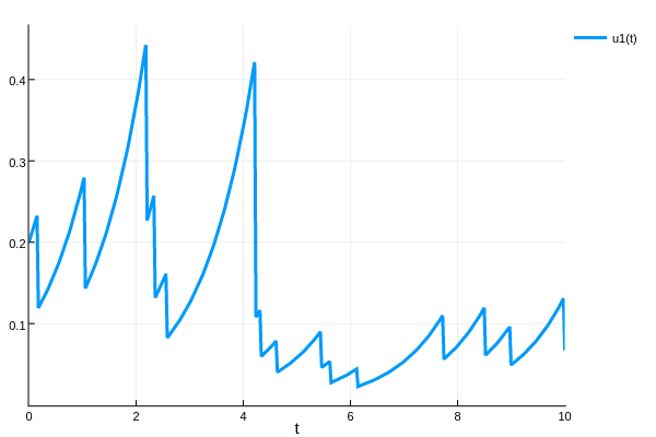
Variable Rate Jumps
Now let's define a jump which is coupled to the differential equation. Let's let the rate be the current value of the solution, that is:
rate = (t,u) -> u[1]Using the same affect!
affect! = (integrator) -> (integrator.u[1] = integrator.u[1]/2)we build a VariableRateJump:
jump = VariableRateJump(rate,affect!)To make things interesting, let's copy this jump:
jump2 = deepcopy(jump)so that way we have two independent jump processes. We now couple these jumps to the ODEProblem:
jump_prob = JumpProblem(prob,Direct(),jump,jump2)which we once again solve using an ODE solver:
sol = solve(jump_prob,Tsit5())
plot(sol)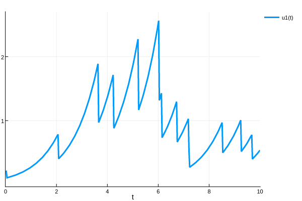
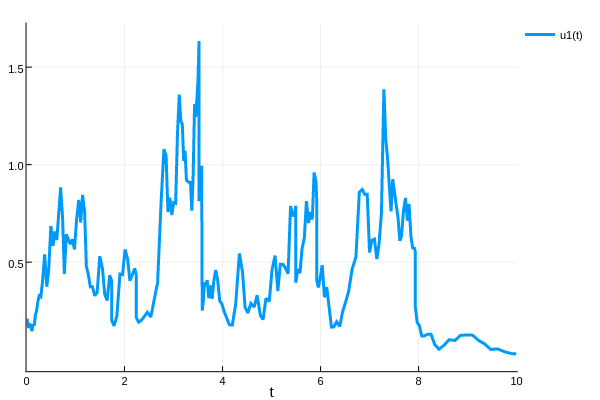
Jump Diffusion
Now we will finally solve the jump diffusion problem. The steps are the same as before, except we now start with a SDEProblem instead of an ODEProblem. Using the same drift function f as before, we add multiplicative noise via:
g = function (t,u,du)
  du[1] = u[1]
end

prob = SDEProblem(f,g,[0.2],(0.0,10.0))
and couple it to the jumps:
jump_prob = JumpProblem(prob,Direct(),jump,jump2)We then solve it using an SDE algorithm:
sol = solve(jump_prob,SRIW1())
plot(sol)