Parallel Monte Carlo Simulations

Performing a Monte Carlo Simulation

To perform a Monte Carlo simulation, you simply use the interface:

sim = monte_carlo_simulation(prob,alg,kwargs...)

The keyword arguments take in the arguments for the common solver interface. The special keyword arguments to note are:

num_monte: The number of simulations to run. Default is 10,000.
prob_func: The function by which the problem is to be modified.
output_func: The reduction function.

One can specify a function prob_func which changes the problem. For example:

function prob_func(prob)
  prob.u0 = randn()*prob.u0
  prob
end

modifies the initial condition for all of the problems by a standard normal random number (a different random number per simulation). This can be used to perform searches over initial values. If your function is a ParameterizedFunction, you can do similar modifications to f to perform a parameter search. The output_func is a reduction function. For example, if we wish to only save the 2nd coordinate at the end of the solution, we can do:

output_func(sol) = sol[end,2]

Parallelism

Since this is using pmap internally, it will use as many processors as you have Julia processes. To add more processes, use addprocs(n). See Julia's documentation for more details.

Solution

The resulting type is a MonteCarloSimulation, which includes the array of solutions. If the problem was a TestProblem, summary statistics on the errors are returned as well.

Plot Recipe

There is a plot recipe for a AbstractMonteCarloSimulation which composes all of the plot recipes for the component solutions. The keyword arguments are passed along. A useful argument to use is linealpha which will change the transparency of the plots.

Example

Let's test the sensitivity of the linear ODE to its initial condition.

addprocs(4)
using DiffEqMonteCarlo, DiffEqBase, DiffEqProblemLibrary, OrdinaryDiffEq
prob = prob_ode_linear
prob_func = function (prob)
  prob.u0 = rand()*prob.u0
  prob
end
sim = monte_carlo_simulation(prob,Tsit5(),prob_func=prob_func,num_monte=100)

using Plots
plotly()
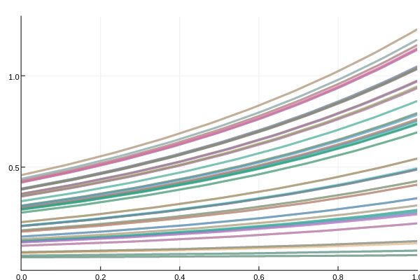
plot(sim,linealpha=0.4)

Here we solve the same ODE 100 times on 4 different cores, jiggling the initial condition by rand(). The resulting plot is as follows:

monte_carlo_plot