Parameter Estimation

Parameter estimation for ODE models is provided by the DiffEq suite. The current functionality includes build_optim_objective and lm_fit. Note these require that the problem is defined using a ParameterizedFunction.

build_optim_objective

build_optim_objective builds an objective function to be used with Optim.jl.

build_optim_objective(prob,tspan,t,data;loss_func = L2DistLoss,kwargs...)

The first argument is the DEProblem to solve. Second is the tspan. Next is t, the set of timepoints which the data is found at. The last argument which is required is the data, which are the values that are known, in order to be optimized against. Optionally, one can choose a loss function from LossFunctions.jl or use the default of an L2 loss. The keyword arguments are passed to the ODE solver.

build_lsoptim_objective

build_lsoptim_objective builds an objective function to be used with LeastSquaresOptim.jl.

build_lsoptim_objective(prob,tspan,t,data;kwargs...)

The arguments are the same as build_optim_objective.

lm_fit

lm_fit is a function for fitting the parameters of an ODE using the Levenberg-Marquardt algorithm. This algorithm is really bad and thus not recommended since, for example, the Optim.jl algorithms on an L2 loss are more performant and robust. However, this is provided for completeness as most other differential equation libraries use an LM-based algorithm, so this allows one to test the increased effectiveness of not using LM.

lm_fit(prob::DEProblem,tspan,t,data,p0;kwargs...)

The arguments are similar to before, but with p0 being the initial conditions for the parameters and the kwargs as the args passed to the LsqFit curve_fit function (which is used for the LM solver). This returns the fitted parameters.

Examples

We choose to optimize the parameters on the Lotka-Volterra equation. We do so by defining the function as a ParmaeterizedFunction:

f = @ode_def_nohes LotkaVolterraTest begin
  dx = a*x - b*x*y
  dy = -c*y + d*x*y
end a=>1.5 b=1.0 c=3.0 d=1.0

u0 = [1.0;1.0]
tspan = (0.0,10.0)
prob = ODEProblem(f,u0,tspan)

Notice that since we only used => for a, it's the only free parameter. We create data using the numerical result with a=1.5:

sol = solve(prob,Tsit5())
t = collect(linspace(0,10,200))
randomized = [(sol(t[i]) + .01randn(2)) for i in 1:length(t)]
using RecursiveArrayTools
data = vecvec_to_mat(randomized)

Here we used vecvec_to_mat from RecursiveArrayTools.jl to turn the result of an ODE into a matrix.

If we plot the solution with the parameter at a=1.42, we get the following:

Parameter Estimation Not Fit

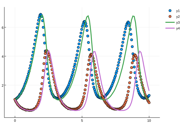
Notice that after one period this solution begins to drift very far off: this problem is sensitive to the choice of a.

To build the objective function for Optim.jl, we simply call the build_optim_objective funtion:

cost_function = build_optim_objective(prob,t,data,Tsit5(),maxiters=10000)

Note that we set maxiters so that way the differential equation solvers would error more quickly when in bad regions of the parameter space, speeding up the process. Now this cost function can be used with Optim.jl in order to get the parameters. For example, we can use Brent's algorithm to search for the best solution on the interval [0,10] by:

using Optim
result = optimize(cost_function, 0.0, 10.0)

This returns result.minimum[1]==1.5 as the best parameter to match the data. When we plot the fitted equation on the data, we receive the following:

Parameter Estimation Fit

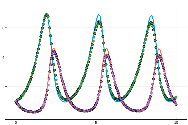
Thus we see that after fitting, the lines match up with the generated data and receive the right parameter value.

We can also use the multivariate optimization functions. For example, we can use the BFGS algorithm to optimize the parameter starting at a=1.42 using:

result = optimize(cost_function, [1.42], BFGS())

Note that some of the algorithms may be sensitive to the initial condition. For more details on using Optim.jl, see the documentation for Optim.jl.

Lastly, we can use the same tools to estimate multiple parameters simultaneously. Let's use the Lotka-Volterra equation with all parameters free:

f2 = @ode_def_nohes LotkaVolterraAll begin
  dx = a*x - b*x*y
  dy = -c*y + d*x*y
end a=>1.5 b=>1.0 c=>3.0 d=>1.0

u0 = [1.0;1.0]
tspan = (0.0,10.0)
prob = ODEProblem(f2,u0,tspan)

To solve it using LeastSquaresOptim.jl, we use the build_lsoptim_objective function:

cost_function = build_lsoptim_objective(prob,t,data,Tsit5()))

The result is a cost function which can be used with LeastSquaresOptim. For more details, consult the documentation for LeastSquaresOptim.jl:

x = [1.3,0.8,2.8,1.2]
res = optimize!(LeastSquaresProblem(x = x, f! = cost_function,
                output_length = length(t)*length(prob.u0)),
                LeastSquaresOptim.Dogleg(),LeastSquaresOptim.LSMR(),
                ftol=1e-14,xtol=1e-15,iterations=100,grtol=1e-14)

We can see the results are:

println(res.minimizer)

Results of Optimization Algorithm
 * Algorithm: Dogleg
 * Minimizer: [1.4995074428834114,0.9996531871795851,3.001556360700904,1.0006272074128821]
 * Sum of squares at Minimum: 0.035730
 * Iterations: 63
 * Convergence: true
 * |x - x'| < 1.0e-15: true
 * |f(x) - f(x')| / |f(x)| < 1.0e-14: false
 * |g(x)| < 1.0e-14: false
 * Function Calls: 64
 * Gradient Calls: 9
 * Multiplication Calls: 135

and thus this algorithm was able to correctly identify all four parameters.