Differential Algebraic Equations

This tutorial will introduce you to the functionality for solving DAEs. Other introductions can be found by checking out DiffEqTutorials.jl.

In this example we will solve the implicit ODE equation

where f is the a variant of the Roberts equation. This equations is actually of the form

or is also known as a constrained differential equation where g is the constraint equation. The Roberts model can be written in the form:

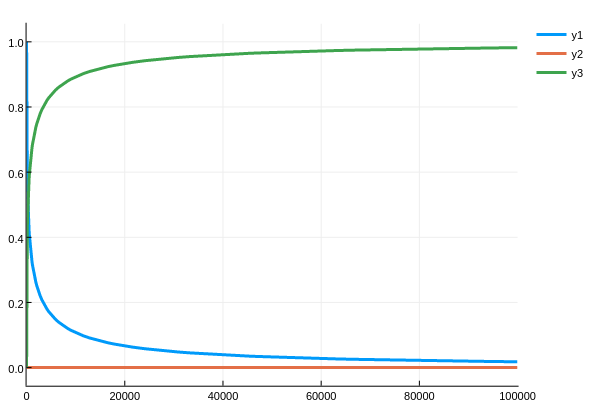
with initial conditions $y_1(0) = 1$, $y_2(0) = 0$, $y_3(0) = 0$, $dy_1 = - 0.04$, $dy_2 = 0.04$, and $dy_3 = 0.0$.

The workflow for DAEs is the same as for the other types of equations, where all you need to know is how to define the problem. A DAEProblem is specified by defining an in-place update f(t,u,du,out) which uses the values to mutate out as the output. To makes this into a DAE, we move all of the variables to one side. Thus we can define the function:

f = function (t,u,du,out)
  out[1] = - 0.04u[1]              + 1e4*u[2]*u[3] - du[1]
  out[2] = + 0.04u[1] - 3e7*u[2]^2 - 1e4*u[2]*u[3] - du[2]
  out[3] = u[1] + u[2] + u[3] - 1.0
end

with initial conditons

u₀ = [1.0, 0, 0]
du₀ = [-0.04, 0.04, 0.0]
tspan = (0.0,100000.0)

and make the DAEProblem:

using DifferentialEquations
prob = DAEProblem(f,u₀,du₀,tspan)

As with the other DifferentialEquations problems, the commands are then to solve and plot. Here we will use the IDA solver from Sundials:

sol = solve(prob,IDA())
using Plots; plotly() # Using the Plotly backend
plot(sol)

which, despite how interesting the model looks, produces a relatively simple output: