Stochastic Differential Equations
This tutorial will introduce you to the functionality for solving SDE. Other introductions can be found by checking out DiffEqTutorials.jl.
Basics
In this example we will solve the equation
where $f(t,u)=αu$ and $g(t,u)=βu$. We know via Stochastic Calculus that the solution to this equation is $u(t,W)=u₀\exp((α-\frac{β^2}{2})t+βW)$. To solve this numerically, we define a problem type by giving it the equation and the initial condition:
using DifferentialEquations
α=1
β=1
u₀=1/2
f(t,u) = α*u
g(t,u) = β*u
dt = 1//2^(4)
tspan = (0.0,1.0)
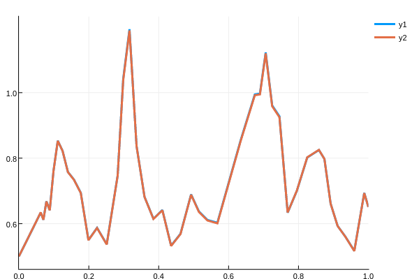
prob = SDEProblem(f,g,u₀,(0.0,1.0))The solve interface is then the same as with ODEs. Here we will use the classic Euler-Maruyama algorithm EM and plot the solution:
sol = solve(prob,EM(),dt=dt)
using Plots; plotly() # Using the Plotly backend
plot(sol)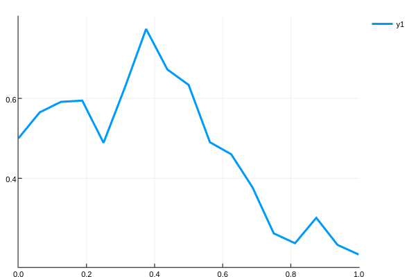
Higher Order Methods
One unique feature of DifferentialEquations.jl is that higher-order methods for stochastic differential equations are included. For reference, let's also give the SDEProblem the analytical solution. We can do this by making a test problem. This can be a good way to judge how accurate the algorithms are, or is used to test convergence of the algorithms for methods developers. Thus we define the problem object with:
analytic(t,u₀,W) = u₀*exp((α-(β^2)/2)*t+β*W)
prob = SDETestProblem(f,g,u₀,analytic)
and then we pass this information to the solver and plot:
#We can plot using the classic Euler-Maruyama algorithm as follows:
sol =solve(prob,EM(),dt=dt)
plot(sol,plot_analytic=true)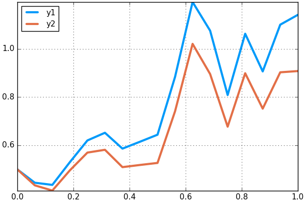
We can choose a higher-order solver for a more accurate result:
sol =solve(prob,SRIW1(),dt=dt,adaptive=false)
plot(sol,plot_analytic=true)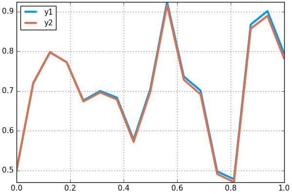
By default, the higher order methods have adaptivity. Thus one can use
sol =solve(prob,SRIW1())
plot(sol,plot_analytic=true)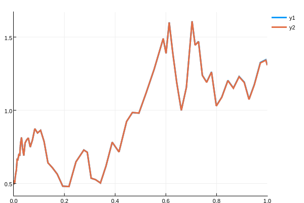
Here we allowed the solver to automatically determine a starting dt. This estimate at the beginning is conservative (small) to ensure accuracy. We can instead start the method with a larger dt by passing in a value for the starting dt:
sol =solve(prob,SRIW1(),dt=dt)
plot(sol,plot_analytic=true)