Event Handling and Callback Functions

Introduction to Callback Functions

DifferentialEquations.jl allows for using callback functions to inject user code into the solver algorithms. It allows for safely and accurately applying events and discontinuities. Multiple callbacks can be chained together, and these callback types can be used to build libraries of extension behavior.

The Callback Types

The callback types are defined as follows. There are two callback types: the ContinuousCallback and the DiscreteCallback. The ContinuousCallback is applied when a continuous condition function hits zero. This type of callback implements what is known in other problem solving environments as an Event. A DiscreteCallback is applied when its condition function is true.

ContinuousCallbacks

ContinuousCallback(condition,affect!,
                   rootfind,
                   save_positions;
                   affect_neg! = affect!,
                   interp_points=10,
                   abstol=1e-14,reltol=0)

The arguments are defined as follows:

condition: This is a function condition(t,u,integrator) for declaring when the callback should be used. A callback is initiated if the condition hits 0 within the time interval.
affect!: This is the function affect!(integrator) where one is allowed to modify the current state of the integrator. For more information on what can be done, see the Integrator Interface manual page.
rootfind: This is a boolean for whether to rootfind the event location. If this is set to true, the solution will be backtracked to the point where condition==0. Otherwise the systems and the affect! will occur at t+dt.
interp_points: The number of interpolated points to check the condition. The condition is found by checking whether any interpolation point / endpoint has a different sign. If interp_points=0, then conditions will only be noticed if the sign of condition is different at t than at t+dt. This behavior is not robust when the solution is oscillatory, and thus it's recommended that one use some interpolation points (they're cheap to compute!).
save_positions: Boolean tuple for whether to save before and after the affect!. The first save will always occcur (if true), and the second will only occur when an event is detected. For discontinuous changes like a modification to u to be handled correctly (without error), one should set save_positions=(true,true).

Additionally, keyword arguments for abstol and reltol can be used to specify a tolerance from zero for the rootfinder: if the starting condition is less than the tolerance from zero, then no root will be detected. This is to stop repeat events happening just after a previously rootfound event. The default has abstol=1e-14 and reltol=0.

DiscreteCallback

DiscreteCallback(condition,affect!,save_positions)

condition: This is a function condition(t,u,integrator) for declaring when the callback should be used. A callback is initiated if the condition evaluates to true.
affect!: This is the function affect!(integrator) where one is allowed to modify the current state of the integrator. For more information on what can be done, see the Integrator Interface manual page.
save_positions: Boolean tuple for whether to save before and after the affect!. The first save will always occcur (if true), and the second will only occur when an event is detected. For discontinuous changes like a modification to u to be handled correctly (without error), one should set save_positions=(true,true).

CallbackSet

Multiple callbacks can be chained together to form a CallbackSet. A CallbackSet is constructed by passing the constructor ContinuousCallback, DiscreteCallback, or other CallbackSet instances:

CallbackSet(cb1,cb2,cb3)

You can pass as many callbacks as you like. When the solvers encounter multiple callbacks, the following rules apply:

ContinuousCallbacks are applied before DiscreteCallbacks. (This is because they often implement event-finding that will backtrack the timestep to smaller than dt).
For ContinuousCallbacks, the event times are found by rootfinding and only the first ContinuousCallback affect is applied.
The DiscreteCallbacks are then applied in order. Note that the ordering only matters for the conditions: if a previous callback modifies u in such a way that the next callback no longer evaluates condition to true, its affect will not be applied.

Using Callbacks

The callback type is then sent to the solver (or the integrator) via the callback keyword argument:

sol = solve(prob,alg,callback=cb)

You can supply nothing, a single DiscreteCallback or ContinuousCallback, or a CallbackSet.

Note About Saving

When a callback is supplied, the default saving behavior is turned off. This is because otherwise events would "double save" one of the values. To re-enable the standard saving behavior, one must have the first save_positions value be true for at least one callback.

DiscreteCallback Examples

Example 1: AutoAbstol

MATLAB's Simulink has the option for an automatic absolute tolerance. In this example we will implement a callback which will add this behavior to any JuliaDiffEq solver which implments the integrator and callback interface.

The algorithm is as follows. The default value is set to start at 1e-6, though we will give the user an option for this choice. Then as the simulation progresses, at each step the absolute tolerance is set to the maximum value that has been reached so far times the relative tolerance. This is the behavior that we will implement in affect!.

Since the effect is supposed to occur every timestep, we use the trivial condition:

condition = function (t,u,integrator)
    true
end

which always returns true. For our effect we will overload the call on a type. This type will have a value for the current maximum. By doing it this way, we can store the current state for the running maximum. The code is as follows:

type AutoAbstolAffect{T}
  curmax::T
end
# Now make `affect!` for this:
function (p::AutoAbstolAffect)(integrator)
  p.curmax = max(p.curmax,integrator.u)
  integrator.opts.abstol = p.curmax * integrator.opts.reltol
  u_modified!(integrator,false)
end

This makes affect!(integrator) use an internal mutating value curmax to update the absolute tolerance of the integrator as the algorithm states.

Lastly, we can wrap it in a nice little constructor:

function AutoAbstol(save=true;init_curmax=1e-6)
  affect! = AutoAbstolAffect(init_curmax)
  condtion = (t,u,integrator) -> true
  save_positions = (save,false)
  DiscreteCallback(condtion,affect!,save_positions)
end

This creates the DiscreteCallback from the affect! and condition functions that we implemented. Now

cb = AutoAbstol(save=true;init_curmax=1e-6)

returns the callback that we created. We can then solve an equation using this by simply passing it with the callback keyword argument. Using the integrator interface rather than the solve interface, we can step through one by one to watch the absolute tolerance increase:

integrator = init(prob,BS3(),callback=cb)
at1 = integrator.opts.abstol
step!(integrator)
at2 = integrator.opts.abstol
@test at1 < at2
step!(integrator)
at3 = integrator.opts.abstol
@test at2 < at3

Note that this example is contained in DiffEqCallbacks.jl, a library of useful callbacks for JuliaDiffEq solvers.

ContinuousCallback Examples

Example 1: Bouncing Ball

Let's look at the bouncing ball. @ode_def from ParameterizedFunctions.jl was to define the problem, where the first variable y is the height which changes by v the velocity, where the velocity is always changing at -g which is the gravitational constant. This is the equation:

f = @ode_def BallBounce begin
  dy =  v
  dv = -g
end g=9.81

All we have to do in order to specify the event is to have a function which should always be positive with an event occurring at 0. For now at least that's how it's specified. If a generalization is needed we can talk about this (but it needs to be "root-findable"). For here it's clear that we just want to check if the ball's height ever hits zero:

function condition(t,u,integrator) # Event when event_f(t,u) == 0
  u[1]
end

Notice that here we used the values u instead of the value from the integrator. This is because the values t,u will be appropriately modified at the interpolation points, allowing for the rootfinding behavior to occur.

Now we have to say what to do when the event occurs. In this case we just flip the velocity (the second variable)

function apply_event!(integrator)
  integrator.u[2] = -integrator.u[2]
end

For safety, we use interp_points=10. We will enable rootfind because this means that when an event is detected, the solution will be approriately backtracked to the exact time at which the ball hits the floor. Lastly, since we are applying a discontinuous change, we set save_values=(true,true) so that way at the event location t, the solution for the velocity will be left continuous and then jump at t to start solving again (and the interpolations will work). The callback is thus specified by:

interp_points = 10
rootfind = true
save_positions = (true,true)
cb = Callback(condtion,affect!,rootfind,interp_points,save_positions)

Then you can solve and plot:

u0 = [50.0,0.0]
tspan = (0.0,15.0)
prob = ODEProblem(f,u0,tspan)
sol = solve(prob,Tsit5(),callback=cb)
plot(sol)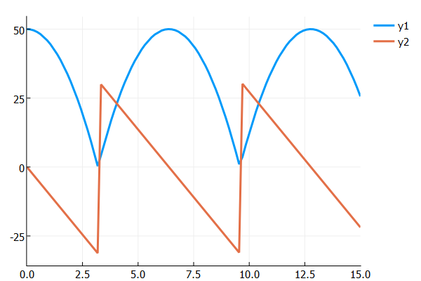

BallBounce

As you can see from the resulting image, DifferentialEquations.jl is smart enough to use the interpolation to hone in on the time of the event and apply the event back at the correct time. Thus one does not have to worry about the adaptive timestepping "overshooting" the event as this is handled for you. Notice that the event macro will save the value(s) at the discontinuity.

Example 2: Growing Cell Population

Note

This example will not work on the current version due to the changes in the callback infrustructure. This message will be removed when that is no longer the case.

Another interesting issue is with models of changing sizes. The ability to handle such events is a unique feature of DifferentialEquations.jl! The problem we would like to tackle here is a cell population. We start with 1 cell with a protein X which increases linearly with time with rate parameter α. Since we are going to be changing the size of the population, we write the model in the general form:

const α = 0.3
f = function (t,u,du)
  for i in 1:length(u)
    du[i] = α*u[i]
  end
end

Our model is that, whenever the protein X gets to a concentration of 1, it triggers a cell division. So we check to see if any concentrations hit 1:

function condition(t,u,integrator) # Event when event_f(t,u) == 0
  1-maximum(u)
end

Again, recall that this function finds events as switching from positive to negative, so 1-maximum(u) is positive until a cell has a concentration of X which is 1, which then triggers the event. At the event, we have that the cell splits into two cells, giving a random amount of protein to each one. We can do this by resizing the cache (adding 1 to the length of all of the caches) and setting the values of these two cells at the time of the event:

function affect!(integrator)
  resize!(integrator,length(integrator.u)+1)
  maxidx = findmax(u)[2]
  Θ = rand()
  u[maxidx] = Θ
  u[end] = 1-Θ
end

As noted in the Integrator Interface, resize!(integrator,length(integrator.u)+1) is used to change the length of all of the internal caches (which includes u) to be their current length + 1, growing the ODE system. Then the following code sets the new protein concentrations. Now we can solve:

interp_points = 10
rootfind = true
save_positions = (true,true)
cb = Callback(condtion,affect!,rootfind,interp_points,save_positions)
u0 = [0.2]
tspan = (0.0,10.0)
prob = ODEProblem(f,u0,tspan)
sol = solve(prob,callback=callback)

The plot recipes do not have a way of handling the changing size, but we can plot from the solution object directly. For example, let's make a plot of how many cells there are at each time. Since these are discrete values, we calculate and plot them directly:

plot(sol.t,map((x)->length(x),sol[:]),lw=3,
     ylabel="Number of Cells",xlabel="Time")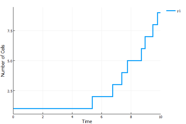

NumberOfCells

Now let's check-in on a cell. We can still use the interpolation to get a nice plot of the concentration of cell 1 over time. This is done with the command:

ts = linspace(0,10,100)
plot(ts,map((x)->x[1],sol.(ts)),lw=3,
     ylabel="Amount of X in Cell 1",xlabel="Time")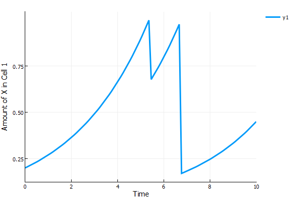

Cell1

Notice that every time it hits 1 the cell divides, giving cell 1 a random amount of X which then grows until the next division.

Note that one macro which was not shown in this example is @ode_change_deleteat which performs deleteat! on the caches. For example, to delete the second cell, we could use:

deleteat!(integrator,2)

This allows you to build sophisticated models of populations with births and deaths.