Uncertainty Quantification
Uncertainty quantification allows a user to identify the uncertainty associated with the numerical approximation given by DifferentialEquations.jl. This page describes the different methods available for quanitifying such uncertainties.
Note
Since this is currently a work in progress, the package DiffEqUncertainty.jl which contains this functionality is currently unregistered and has to be installed via:
Pkg.clone("https://github.com/JuliaDiffEq/DiffEqUncertainty.jl")ProbInts
The ProbInts method for uncertainty quantification involves the transformation of an ODE into an associated SDE where the noise is related to the timesteps and the order of the algorithm. This is implemented into the DiffEq system via a callback function:
ProbIntsUncertainty(σ,order,save=true)σ is the noise scaling factor and order is the order of the algorithm. save is for choosing whether this callback should control the saving behavior. Generally this is true unless one is stacking callbacks in a CallbackSet.
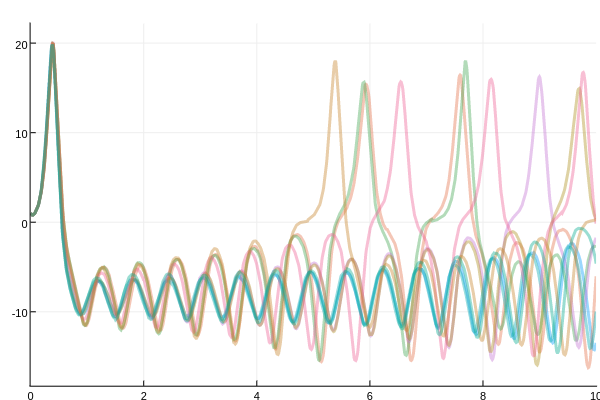
Example
To use the callback, we simply create it and pass it to the solver. Here I will use DiffEqMonteCarlo in order to perform the simulation 10 times and plot the results together.
using DiffEqUncertainty, DiffEqBase, OrdinaryDiffEq, DiffEqProblemLibrary, DiffEqMonteCarlo
using Base.Test

using ParameterizedFunctions
g = @ode_def_bare LorenzExample begin
  dx = σ*(y-x)
  dy = x*(ρ-z) - y
  dz = x*y - β*z
end σ=>10.0 ρ=>28.0 β=(8/3)
u0 = [1.0;0.0;0.0]
tspan = (0.0,10.0)
prob = ODEProblem(g,u0,tspan)

cb = ProbIntsUncertainty(1e4,5)
solve(prob,Tsit5())
sim = monte_carlo_simulation(prob,Tsit5(),num_monte=10,callback=cb,adaptive=false,dt=1/10)

using Plots; plotly(); plot(sim,vars=(0,1),linealpha=0.4)