Integrator Interface
The integrator interface gives one the ability to interactively step through the numerical solving of a differential equation. Through this interface, one can easily monitor results, modify the problem during a run, and dynamically continue solving as one sees fit.
Note: this is currently only offered by OrdinaryDiffEq.jl, DelayDiffEq.jl, and StochasticDiffEq.jl. Solvers from other packages will support this in the near future.
Initialization and Stepping
To initialize an integrator, use the syntax:
integrator = init(prob,alg;kwargs...)The keyword args which are accepted are the same Common Solver Options used by solve. The type which is returned is the integrator. One can manually choose to step via the step! command:
step!(integrator)which will take one successful step. This type also implements an integrator interface, so one can step n times (or to the last tstop) using the take iterator:
for i in take(integrator,n) endOne can loop to the end by using solve!(integrator) or using the integrator interface:
for i in integrator endIn addition, some helper iterators are provided to help monitor the solution. For example, the tuples iterator lets you view the values:
for (t,u) in tuples(integrator)
  @show t,u
end
and the intervals iterator lets you view the full interval:
for (tprev,uprev,t,u) in intervals(integrator)
  @show tprev,t
end
Lastly, one can dynamically control the "endpoint". The initialization simply makes prob.tspan[2] the last value of tstop, and many of the iterators are made to stop at the final tstop value. However, step! will always take a step, and one can dynamically add new values of tstops by modifiying the variable in the options field: push!(integrator.opts.tstops,new_t).
Handing Integrators
The integrator type holds all of the information for the intermediate solution of the differential equation. Useful fields are:
t- time of the proposed stepu- value at the proposed stepuserdata- user-provided data typeopts- common solver optionsalg- the algorithm associated with the solutionf- the function being solvedsol- the current state of the solutiontprev- the last timepointuprev- the value at the last timepoint
The userdata is the type which is provided by the user as a keyword arg in init. opts holds all of the common solver options, and can be mutated to change the solver characteristics. For example, to modify the absolute tolerance for the future timesteps, one can do:
integrator.opts.abstol = 1e-9The sol field holds the current solution. This current solution includes the interpolation function if available, and thus integrator.sol(t) lets one interpolate efficiently over the whole current solution. Additionally, a a "current interval interpolation function" is provided on the integrator type via integrator(t). This uses only the solver information from the interval [tprev,t] to compute the interpolation, and is allowed to extrapolate beyond that interval.
Note about mutating
Be cautious: one should not directly mutate the t and u fields of the integrator. Doing so will destroy the accuracy of the interpolator and can harm certain algorithms. Instead if one wants to introduce discontinuous changes, one should use the Event Handling and Callback Functions. Modifications within a callback affect! surrounded by saves provides an error-free handling of the discontinuity.
Integrator vs Solution
The integrator and the solution have very different actions because they have very different meanings. The Solution type is a type with history: it stores all of the (requested) timepoints and interpolates/acts using the values closest in time. On the other hand, the Integrator type is a local object. It only knows the times of the interval it currently spans, the current caches and values, and the current state of the solver (the current options, tolerances, etc.). These serve very different purposes:
The
integrator's interpolation can extrapolate, both forward and backward in in time. This is used to estimate events and is internally used for predictions.The
integratoris fully mutable upon iteration. This means that every time an iterator affect is used, it will take timesteps from the current time. This means thatfirst(integrator)!=first(integrator)since theintegratorwill step once to evaluate the left and then step once more (not backtracking). This allows the iterator to keep dynamically stepping, though one should note that it may violate some immutablity assumptions commonly made about iterators.
If one wants the solution object, then one can find it in integrator.sol.
Function Interface
In addition to the type interface, a function interface is provided which allows for safe modifications of the integrator type, and allows for uniform usage throughout the ecosystem (for packages/algorithms which implement the functions). The following functions make up the interface:
Saving Controls
savevalues!(integrator): Adds the current state to thesol.
Cache Iterators
user_cache(integrator): Returns an iterator over the user-facing cache arrays.u_cache(integrator): Returns an iterator over the cache arrays foruin the method. This can be used to change internal values as needed.du_cache(integrator): Returns an iterator over the cache arrays for rate quantities the method. This can be used to change internal values as needed.full_cache(integrator): Returns an iterator over the cache arrays of the method. This can be used to change internal values as needed.
Stepping Controls
u_modified!(integrator,bool): Bool which states whether a change touoccurred, allowing the solver to handle the discontinuity. By default, this is assumed to be true if a callback is used. This will result in the re-calculation of the derivative att+dt, which is not necessary if the algorithm is FSAL andudoes not experience a discontinuous change at the end of the interval. Thus ifuis unmodified in a callback, a single call to the derivative calculation can be eliminated byu_modified!(integrator,false).get_proposed_dt(integrator,factor): Gets the proposeddtfor the next timestep.set_proposed_dt!(integrator,factor): Sets the proposeddtfor the next timestep.proposed_dt(integrator): Returns thedtof the proposed step.terminate!(integrator): Terminates the integrator by emptyingtstops. This can be used in events and callbacks to immediately end the solution process.change_t_via_interpolation(integrator,t,modify_save_endpoint=Val{false}): This option lets one modify the currenttand changes all of the corresponding values using the local interpolation. If the current solution has already been saved, one can provide the optional valuemodify_save_endpointto also modify the endpoint ofsolin the same manner.
Resizing
resize!(integrator,k): Resizes the DE to a sizek. This chops off the end of the array, or adds blank values at the end, depending on whetherk>length(integrator.u).resize_non_user_cache!(integrator,k): Resizes the non-user facing caches to be compatible with a DE of sizek. This includes resizing Jacobian caches. Note that in many cases,resize!simple resizesuser_cachevariables and then calls this function. This finer control is required for someAbstractArrayoperations.deleteat_non_user_cache!(integrator,idxs):deleteat!s the non-user facing caches at indicesidxs. This includes resizing Jacobian caches. Note that in many cases,deleteat!simpledeleteat!suser_cachevariables and then calls this function. This finer control is required for someAbstractArrayoperations.addat_non_user_cache!(integrator,idxs):addat!s the non-user facing caches at indicesidxs. This includes resizing Jacobian caches. Note that in many cases,addat!simpleaddat!suser_cachevariables and then calls this function. This finer control is required for someAbstractArrayoperations.deleteat!(integrator,idxs): Shrinks the ODE by deleting theidxscomponents.addat!(integrator,idxs): Grows the ODE by adding theidxscomponents. Must be contiguous indices.
Misc
get_du(integrator): Returns the derivative att.
Note
Note that not all of these functions will be implemented for every algorithm. Some have hard limitations. For example, Sundials.jl cannot resize problems. When a function is not limited, an error will be thrown.
Additional Options
The following options can additionally be specified in init (or be mutated in the opts) for further control of the integrator:
advance_to_tstop: This makesstep!continue to the next value intstop.stop_at_next_tstop: This forces the iterators to stop at the next value oftstop.
For example, if one wants to iterate but only stop at specific values, one can choose:
integrator = init(prob,Tsit5();dt=1//2^(4),tstops=[0.5],advance_to_tstop=true)
for (t,u) in tuples(integrator)
  @test t ∈ [0.5,1.0]
end
which will only enter the loop body at the values in tstops (here, prob.tspan[2]==1.0 and thus there are two values of tstops which are hit). Addtionally, one can solve! only to 0.5 via:
integrator = init(prob,Tsit5();dt=1//2^(4),tstops=[0.5])
integrator.opts.stop_at_next_tstop = true
solve!(integrator)
Plot Recipe
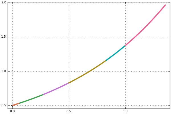
Like the Solution type, a plot recipe is provided for the Integrator type. Since the Integrator type is a local state type on the current interval, plot(integrator) returns the solution on the current interval. The same options for the plot recipe are provided as for sol, meaning one can choose variables via the vars keyword argument, or change the plotdensity / turn on/off denseplot.
Additionally, since the integrator is an integrator, this can be used in the Plots.jl animate command to iteratively build an animation of the solution while solving the differential equation.
For an example of manually chaining together the iterator interface and plotting, one should try the following:
using DifferentialEquations, DiffEqProblemLibrary, Plots
prob = prob_ode_linear

using Plots
integrator = init(prob,Tsit5();dt=1//2^(4),tstops=[0.5])
pyplot(show=true)
plot(integrator)
for i in integrator
  display(plot!(integrator,vars=(0,1),legend=false))
end
step!(integrator); plot!(integrator,vars=(0,1),legend=false)
savefig("iteratorplot.png")