Plot Functions

Standard Plots

Plotting functionality is provided by recipes to Plots.jl. To use plot solutions, simply call the plot(type) after importing Plots.jl and the plotter will generate appropriate plots.

#Pkg.add("Plots") # You need to install Plots.jl before your first time using it!
using Plots
plot(sol) # Plots the solution

Many of the types defined in the DiffEq universe, such as ODESolution, ConvergenceSimulationWorkPrecision, etc. have plot recipes to handle the default plotting behavior. Plots can be customized using all of the keyword arguments provided by Plots.jl. For example, we can change the plotting backend to the GR package and put a title on the plot by doing:

gr()
plot(sol,title="I Love DiffEqs!")

Density

If the problem was solved with dense=true, then denseplot controls whether to use the dense function for generating the plot, and plotdensity is the number of evenly-spaced points (in time) to plot. For example:

plot(sol,denseplot=false)

means "only plot the points which the solver stepped to", while:

plot(sol,plotdensity=1000)

means to plot 1000 points using the dense function (since denseplot=true by default).

Choosing Variables

In the plot command, one can choose the variables to be plotted in each plot. The master form is:

vars = [(f1,0,1), (f2,1,3), (f3,4,5)]

where this would mean plot f1(variable 1, variable 2), f2(variable 1, variable 3), f3(variable 4, variable 5) all on the same graph. (0 is considered to be time, or the independent variable). The function f1 should take in scalars and return a tuple. If no function is given, for example,

vars = [(0,1), (1,3), (4,5)]

where this would mean plot variable 0 vs 1, 1 vs 3, and 4 vs 5 all on the same graph. While this can be used for everything, the following conveniences are provided:

Everywhere in a tuple position where we only find an integer, this variable is plotted as a function of time. For example, the list above is equivalent to:

vars = [1, (1,3), (4,5)]

and

vars = [1, 3, 4]

is the most concise way to plot the variables 1, 3, and 4 as a function of time.

It is possible to omit the list if only one plot is wanted: (2,3) and 4 are respectively equivalent to [(2,3)] and [(0,4)].
A tuple containing one or several lists will be expanded by associating corresponding elements of the lists with each other:

vars = ([1,2,3], [4,5,6])

is equivalent to

vars = [(1,4), (2,5), (3,6)]

and

vars = (1, [2,3,4])

is equivalent to

vars = [(1,2), (1,3), (1,4)]

Instead of using integers, one can use the symbols from a ParameterizedFunction. For example, vars=(:x,:y) will replace the symbols with the integer values for components :x and :y.
n-dimensional groupings are allowed. For example, (1,2,3,4,5) would be a 5-dimensional plot between the associated variables.

Complex Numbers and High Dimensional Plots

The recipe library DimensionalPlotRecipes.jl is provided for extra functionality on high dimensional numbers (complex numbers) and other high dimensional plots. See the README for more details on the extra controls that exist.

Example

using DifferentialEquations, Plots
lorenz = @ode_def Lorenz begin
  dx = σ*(y-x)
  dy = ρ*x-y-x*z
  dz = x*y-β*z
end σ = 10. β = 8./3. ρ => 28.

u0 = [1., 5., 10.]
tspan = (0., 100.)
prob = ODEProblem(lorenz, u0, tspan)
sol = solve(prob)

xyzt = plot(sol, plotdensity=10000,lw=1.5)
xy = plot(sol, plotdensity=10000, vars=(:x,:y))
xz = plot(sol, plotdensity=10000, vars=(:x,:z))
yz = plot(sol, plotdensity=10000, vars=(:y,:z))
xyz = plot(sol, plotdensity=10000, vars=(:x,:y,:z))
plot(plot(xyzt,xyz),plot(xy, xz, yz, layout=(1,3),w=1), layout=(2,1))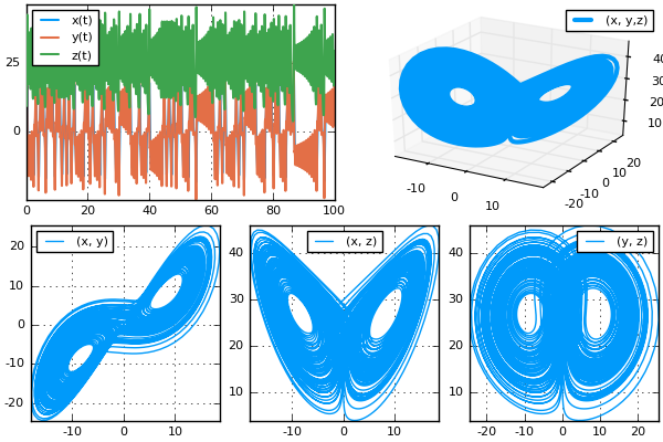

lorenz_plot

An example using the functions:

f(x,y,z) = (sqrt(x^2+y^2+z^2),x)
plot(sol,vars=(f,:x,:y,:z))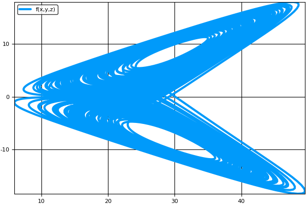

norm_plot

Animations

Using the iterator interface over the solutions, animations can also be generated via the animate(sol) command. One can choose the filename to save to via animate(sol,filename), while the frames per second fps and the density of steps to show every can be specified via keyword arguments. The rest of the arguments will be directly passed to the plot recipe to be handled as normal. For example, we can animate our solution with a larger line-width which saves every 4th frame via:

#Pkg.add("ImageMagick") # You may need to install ImageMagick.jl before your first time using it!
#using ImageMagick # Some installations require using ImageMagick for good animations
animate(sol,lw=3,every=4)

Please see Plots.jl's documentation for more information on the available attributes.