Noise Processes

A NoiseProcess is a type defined as

NoiseProcess(t0,W0,Z0,dist,bridge;
             iip=DiffEqBase.isinplace(dist,3),
             rswm = RSWM())

t0 is the first timepoint
W0 is the first value of the process.
Z0 is the first value of the psudo-process. This is necessary for higher order algorithms. If it's not needed, set to nothing.
dist the distribution for the steps over time.
bridge the bridging distribution. Optional, but required for adaptivity and interpolating at new values.

The signature for the dist is

dist!(rand_vec,W,dt)

for inplace functions, and

rand_vec = dist(W,dt)

otherwise. The signature for bridge is

bridge!(rand_vec,W,W0,Wh,q,h)

and the out of place syntax is

rand_vec = bridge!(W,W0,Wh,q,h)

Here, W is the noise process, W0 is the left side of the current interval, Wh is the right side of the current interval, h is the interval length, and q is the proportion from the left where the interpolation is occuring.

White Noise

The default noise is WHITE_NOISE. This is the noise process which uses randn!. A special dispatch is added for complex numbers for (randn()+im*randn())/sqrt(2). This function is DiffEqBase.wiener_randn (or with ! respectively). Thus its noise function is essentially:

function WHITE_NOISE_DIST(W,dt)
  if typeof(W.dW) <: AbstractArray
    return sqrt(abs(dt))*wiener_randn(size(W.dW))
  else
    return sqrt(abs(dt))*wiener_randn(typeof(W.dW))
  end
end
function WHITE_NOISE_BRIDGE(W,W0,Wh,q,h)
  sqrt((1-q)*q*abs(h))*wiener_randn(typeof(W.dW))+q*(Wh-W0)+W0
end

for the out of place versions, and for the inplace versions

function INPLACE_WHITE_NOISE_DIST(rand_vec,W,dt)
  wiener_randn!(rand_vec)
  rand_vec .*= sqrt(abs(dt))
end
function INPLACE_WHITE_NOISE_BRIDGE(rand_vec,W,W0,Wh,q,h)
  wiener_randn!(rand_vec)
  rand_vec .= sqrt((1.-q).*q.*abs(h)).*rand_vec.+q.*(Wh.-W0).+W0
end

Notice these functions correspond to the distributions for the Wiener process, that is the first one is simply that Brownian steps are distributed N(0,dt), while the second function is the distribution of the Brownian Bridge N(q(Wh-W0)+W0,(1-q)qh). These functions are then placed in a noise process:

NoiseProcess(t0,W0,Z0,WHITE_NOISE_DIST,WHITE_NOISE_BRIDGE,rswm=RSWM())
NoiseProcess(t0,W0,Z0,INPLACE_WHITE_NOISE_DIST,INPLACE_WHITE_NOISE_BRIDGE,rswm=RSWM())

For convenience, the following constructors are predefined:

WienerProcess(t0,W0,Z0=nothing) = NoiseProcess(t0,W0,Z0,WHITE_NOISE_DIST,WHITE_NOISE_BRIDGE,rswm=RSWM())
WienerProcess!(t0,W0,Z0=nothing) = NoiseProcess(t0,W0,Z0,INPLACE_WHITE_NOISE_DIST,INPLACE_WHITE_NOISE_BRIDGE,rswm=RSWM())

These will generate a Wiener process, which can be stepped with step!(W,dt), and interpolated as W(t).

Correlated Noise

One can define a CorrelatedWienerProcess which is a Wiener process with correlations between the Wiener processes. The constructor is:

CorrelatedWienerProcess(Γ,t0,W0,Z0=nothing)
CorrelatedWienerProcess!(Γ,t0,W0,Z0=nothing)

where Γ is the constant covariance matrix.

NoiseWrapper

Another AbstractNoiseProcess is the NoiseWrapper. This produces a new noise process from an old one, which will use its interpolation to generate the noise. This allows you to re-use a previous noise process not just with the same timesteps, but also with new (adaptive) timesteps as well. Thus this is very good for doing Multi-level Monte Carlo schemes and strong convergence testing.

To wrap a noise process, simply use:

NoiseWrapper(W::NoiseProcess)

Example

In this example, we will solve an SDE three times:

First to generate a noise process
Second with the same timesteps to show the values are the same
Third with half-sized timsteps

First we will generate a noise process by solving an SDE:

using StochasticDiffEq,  DiffEqBase, DiffEqNoiseProcess
f1 = (t,u) -> 1.01u
g1 = (t,u) -> 1.01u
dt = 1//2^(4)
prob1 = SDEProblem(f1,g1,1.0,(0.0,1.0))
sol1 = solve(prob1,EM(),dt=dt)

Now we wrap the noise into a NoiseWrapper and solve the same problem:

W2 = NoiseWrapper(sol1.W)
prob1 = SDEProblem(f1,g1,1.0,(0.0,1.0),noise=W2)
sol2 = solve(prob1,EM(),dt=dt)

We can test

@test sol1.u ≈ sol2.u

to see that the values are essentially equal. Now we can use the same process to solve the same trajectory with a smaller dt:

W3 = NoiseWrapper(sol1.W)
prob2 = SDEProblem(f1,g1,1.0,(0.0,1.0),noise=W3)

dt = 1//2^(5)
sol3 = solve(prob2,EM(),dt=dt)

We can plot the results to see what this looks like:

using Plots
plot(sol1)
plot!(sol2)
plot!(sol3)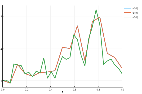

noise_process

In this plot, sol2 covers up sol1 because they hit essentially the same values. You can see that sol3 its similar to the others, because it's using the same underlying noise process just sampled much finer.

To double check, we see that:

plot(sol1.W)
plot!(sol2.W)
plot!(sol3.W)

coupled_wiener

the coupled Wiener processes coincide at every other timepoint, and the intermediate timepoints were calculated according to a Brownian bridge.

Adaptive Example

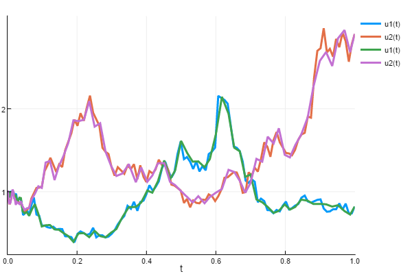
Here we will show that the same noise can be used with the adaptive methods using the NoiseWrapper. SRI and SRIW1 use slightly different error estimators, and thus give slightly different stepping behavior. We can see how they solve the same 2D SDE differently by using the noise wrapper:

prob = SDEProblem(f1,g1,ones(2),(0.0,1.0))
sol4 = solve(prob,SRI(),abstol=1e-8)

W2 = NoiseWrapper(sol4.W)
prob2 = SDEProblem(f1,g1,ones(2),(0.0,1.0),noise=W2)
sol5 = solve(prob2,SRIW1(),abstol=1e-8)

using Plots
plot(sol4)
plot!(sol5)

SRI_SRIW1_diff