Callback Library

DiffEqCallbackLibrary.jl provides a library of various helpful callbacks which can be used with any component solver which implements the callback interface. It adds the following callbacks which are available to users of DifferentialEquations.jl.

Callbacks

Manifold Conservation and Projection

In many cases, you may want to declare a manifold on which a solution lives. Mathematically, a manifold M is defined by a function g as the set of points where g(u)=0. An embedded manifold can be a lower dimensional object which constrains the solution. For example, g(u)=E(u)-C where E is the energy of the system in state u, meaning that the energy must be constant (energy preservation). Thus by defining the manifold the solution should live on, you can retain desired properties of the solution.

It is a consequence of convergence proofs both in the deterministic and stochastic cases that post-step projection to manifolds keep the same convergence rate (stochastic requires a truncation in the proof, details details), thus any algorithm can be easily extended to conserve properties. If the solution is supposed to live on a specific manifold or conserve such property, this guarantees the conservation law without modifying the convergence properties.

Constructor

ManifoldProjection(g;nlsolve=NLSOLVEJL_SETUP(),save=true)

g: The residual function for the manifold: g(u,resid). This is an inplace function which writes to the residual the difference from the manifold components.
nlsolve: A nonlinear solver as defined in the nlsolve format
save: Whether to do the standard saving (applied after the callback)

Example

Here we solve the harmonic oscillator:

u0 = ones(2)
f = function (t,u,du)
  du[1] = u[2]
  du[2] = -u[1]
end
prob = ODEProblem(f,u0,(0.0,100.0))

However, this problem is supposed to conserve energy, and thus we define our manifold to conserve the sum of squares:

function g(u,resid)
  resid[1] = u[2]^2 + u[1]^2 - 2
  resid[2] = 0
end

To build the callback, we just call

cb = ManifoldProjection(g)

Using this callback, the Runge-Kutta method Vern7 conserves energy:

sol = solve(prob,Vern7(),callback=cb)
@test sol[end][1]^2 + sol[end][2]^2 ≈ 2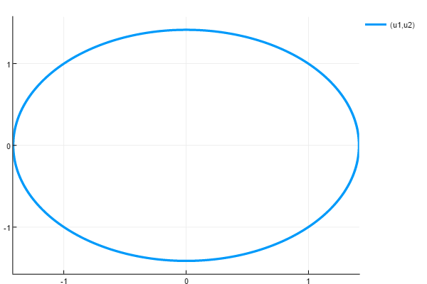

manifold_projection

AutoAbstol

Many problem solving environments such as MATLAB provide a way to automatically adapt the absolute tolerance to the problem. This helps the solvers automatically "learn" what appropriate limits are. Via the callback interface, DiffEqCallbacks.jl implements a callback AutoAbstol which has the same behavior as the MATLAB implementation, that is the absolute tolerance starts and at each iteration it is set to the maximum value that the state has thus far reached times the relative tolerance. If init_curmax is zero, then the initial value is determined by the abstol of the solver. Otherwise this is the initial value for the current maximum abstol.

To generate the callback, use the constructor:

AutoAbstol(save=true;init_curmax=0.0)