Parallel Monte Carlo Simulations

Performing a Monte Carlo Simulation

Building a Problem

To perform a Monte Carlo simulation, define a MonteCarloProblem. The constructor is:

MonteCarloProblem(prob::DEProblem;
                  output_func = (sol,i) -> sol,
                  prob_func= (prob,i)->prob)

• prob_func: The function by which the problem is to be modified.

• output_func: The reduction function.

One can specify a function prob_func which changes the problem. For example:

function prob_func(prob,i)
  prob.u0 = randn()*prob.u0
  prob
end

modifies the initial condition for all of the problems by a standard normal random number (a different random number per simulation). This can be used to perform searches over initial values. Note that the parameter i is a unique counter over the simulations. Thus if you have an array of initial conditions u0_arr, you can have the ith simulation use the ith initial condition via:

function prob_func(prob,i)
  prob.u0 = u0_arr[i]
  prob
end

If your function is a ParameterizedFunction, you can do similar modifications to prob.f to perform a parameter search. The output_func is a reduction function. It's arguments are the generated solution and the unique index for the run. For example, if we wish to only save the 2nd coordinate at the end of each solution, we can do:

output_func(sol,i) = sol[end,2]

Thus the Monte Carlo Simulation would return as its data an array which is the end value of the 2nd dependent variable for each of the runs.

Parameterizing the Monte Carlo Components

The Monte Carlo components can be parameterized by using the ConcreteParameterizedFunction constructors.

ProbParameterizedFunction(prob_func,params)
OutputParameterizedFunction(output_func,params)

Here, the signatures are prob_func(prob,i,params) and output_func(sol,params). These parameters are added to the parameter list for use in the parameter estimation schemes.

Solving the Problem

sim = solve(prob,alg,kwargs...)

The keyword arguments take in the arguments for the common solver interface and will pass them to the differential equation solver. The special keyword arguments to note are:

• num_monte: The number of simulations to run. Default is 10,000.

• parallel_type : The type of parallelism to employ.

The types of parallelism included are:

• :none - No parallelism

• :threads - This uses multithreading. It's local (single computer, shared memory) parallelism only. Fastest when the trajectories are quick.

• :parfor - A multiprocessing parallelism. Slightly better than pmap when the calculations are fast. Does not re-distribute work: each trajectory is assumed to take as long to calculate.

• :pmap - The default. Uses pmap internally. It will use as many processors as you have Julia processes. To add more processes, use addprocs(n). See Julia's documentation for more details. Recommended for the case when each trajectory calculation isn't "too quick" (at least about a millisecond each?).

• :split_threads - This uses threading on each process, splitting the problem into nprocs() even parts. This is for solving many quick trajectories on a multi-node machine. It's recommended you have one process on each node.

Additionally, a MonteCarloEstimator can be supplied

sim = solve(prob,estimator,alg,kwargs...)

These will be detailed when implemented.

Solution

The resulting type is a MonteCarloSimulation, which includes the array of solutions. If the problem was a TestProblem, summary statistics on the errors are returned as well.

Plot Recipe

There is a plot recipe for a AbstractMonteCarloSimulation which composes all of the plot recipes for the component solutions. The keyword arguments are passed along. A useful argument to use is linealpha which will change the transparency of the plots.

Example

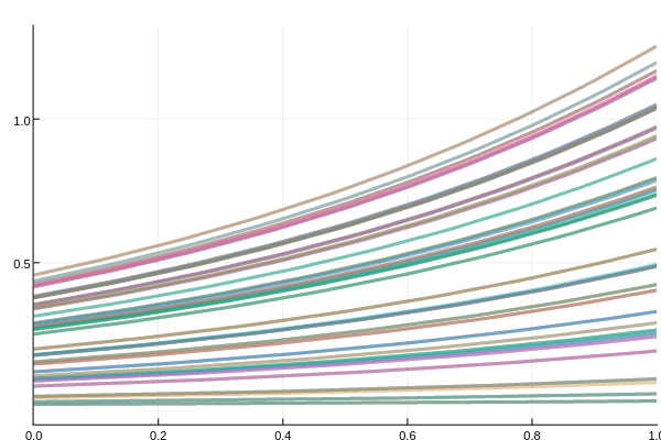
Let's test the sensitivity of the linear ODE to its initial condition.

addprocs(4)
using DiffEqMonteCarlo, DiffEqBase, DiffEqProblemLibrary, OrdinaryDiffEq
prob = prob_ode_linear
prob_func = function (prob)
  prob.u0 = rand()*prob.u0
  prob
end
monte_prob = MonteCarloProblem(prob,prob_func=prob_func)
sim = solve(monte_prob,Tsit5(),num_monte=100)

using Plots
plotly()
plot(sim,linealpha=0.4)

Here we solve the same ODE 100 times on 4 different cores, jiggling the initial condition by rand(). The resulting plot is as follows: