Stochastic Differential Equations

This tutorial will introduce you to the functionality for solving SDEs. Other introductions can be found by checking out DiffEqTutorials.jl. This tutorial assumes you have read the Ordinary Differential Equations tutorial.

Basics

In this example we will solve the equation

where $f(t,u)=αu$ and $g(t,u)=βu$. We know via Stochastic Calculus that the solution to this equation is $u(t,W)=u₀\exp((α-\frac{β^2}{2})t+βW)$. To solve this numerically, we define a problem type by giving it the equation and the initial condition:

using DifferentialEquations
α=1
β=1
u₀=1/2
f(t,u) = α*u
g(t,u) = β*u
dt = 1//2^(4)
tspan = (0.0,1.0)
prob = SDEProblem(f,g,u₀,(0.0,1.0))

The solve interface is then the same as with ODEs. Here we will use the classic Euler-Maruyama algorithm EM and plot the solution:

sol = solve(prob,EM(),dt=dt)
using Plots; plotly() # Using the Plotly backend
plot(sol)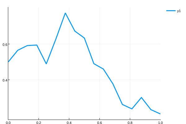

Higher Order Methods

One unique feature of DifferentialEquations.jl is that higher-order methods for stochastic differential equations are included. For reference, let's also give the SDEProblem the analytical solution. We can do this by making a test problem. This can be a good way to judge how accurate the algorithms are, or is used to test convergence of the algorithms for methods developers. Thus we define the problem object with:

analytic(t,u₀,W) = u₀*exp((α-(β^2)/2)*t+β*W)
prob = SDETestProblem(f,g,u₀,analytic)

and then we pass this information to the solver and plot:

#We can plot using the classic Euler-Maruyama algorithm as follows:
sol =solve(prob,EM(),dt=dt)
plot(sol,plot_analytic=true)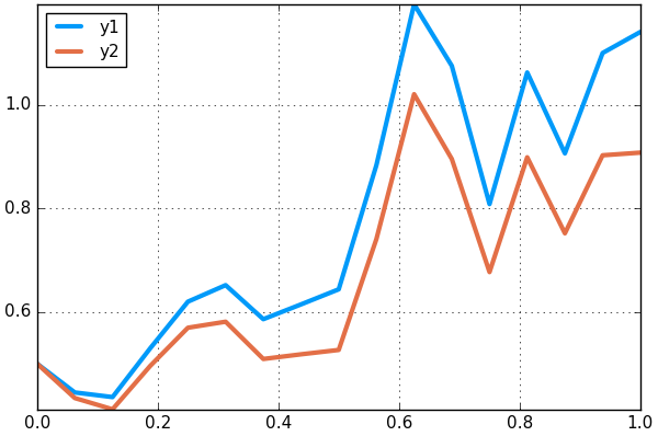

We can choose a higher-order solver for a more accurate result:

sol =solve(prob,SRIW1(),dt=dt,adaptive=false)
plot(sol,plot_analytic=true)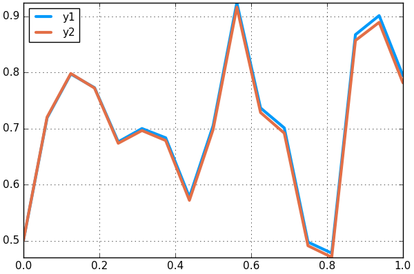

By default, the higher order methods have adaptivity. Thus one can use

sol =solve(prob,SRIW1())
plot(sol,plot_analytic=true)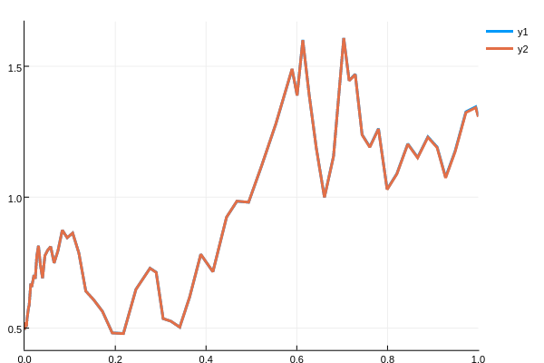

Here we allowed the solver to automatically determine a starting dt. This estimate at the beginning is conservative (small) to ensure accuracy. We can instead start the method with a larger dt by passing in a value for the starting dt:

sol =solve(prob,SRIW1(),dt=dt)
plot(sol,plot_analytic=true)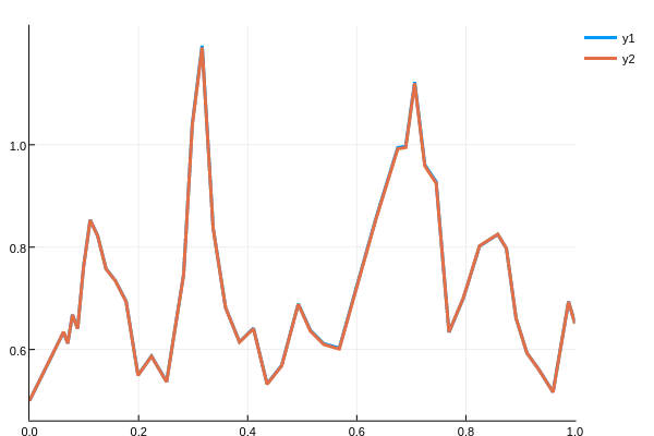

Non-Diagonal Noise

All of the previous examples had diagonal noise, that is a vector of random numbers dW whose size matches the output of g, and the noise is applied element-wise. However, a more general type of noise allows for the terms to linearly mixed.

Let's define a problem with four Wiener processes and two dependent random variables. In this case, we will want the output of g to be a 2x4 matrix, such that the solution is g(t,u)*dW, the matrix multiplication. For example, we can do the following:

f = (t,u,du) -> du.=1.01u
g = function (t,u,du)
  du[1,1] = 0.3u[1]
  du[1,2] = 0.6u[1]
  du[1,3] = 0.9u[1]
  du[1,4] = 0.12u[2]
  du[2,1] = 1.2u[1]
  du[2,2] = 0.2u[2]
  du[2,3] = 0.3u[2]
  du[2,4] = 1.8u[2]
end
prob = SDEProblem(f,g,ones(2),(0.0,1.0),noise_rate_prototype=zeros(2,4))

In our g we define the functions for computing the values of the matrix. The matrix itself is determined by the keyword argument noise_rate_prototype in the SDEProblem constructor. This is a prototype for the type that du will be in g. This can be any AbstractMatrix type. Thus for example, we can define the problem as

# Define a sparse matrix by making a dense matrix and setting some values as not zero
A = zeros(2,4)
A[1,1] = 1
A[1,4] = 1
A[2,4] = 1
sparse(A)

# Make `g` write the sparse matrix values
g = function (t,u,du)
  du[1,1] = 0.3u[1]
  du[1,4] = 0.12u[2]
  du[2,4] = 1.8u[2]
end

# Make `g` use the sparse matrix
prob = SDEProblem(f,g,ones(2),(0.0,1.0),noise_rate_prototype=A)

and now g(t,u) writes into a sparse matrix, and g(t,u)*dW is sparse matrix multiplication.