Improved Branin function

The Branin function is smooth, deterministic, and has three global minima of equal value. That makes it a clean test, but an unrealistic one: a real objective evaluated by simulation is rarely reproducible to the last bit.

The improved Branin function adds a time-varying perturbation inside the cosine term, turning the landscape into something closer to what an optimizer meets in practice:

\[f(x_1, x_2, \tau) = \left(x_2 - \frac{5.1}{4\pi^2}x_1^2 + \frac{5}{\pi}x_1 - 6\right)^2 + 10\left(1 - \frac{1}{8\pi}\right)\cos(x_1 + \tau\,\xi) + 10, \qquad \xi \sim \mathcal{N}(0, 1)\]

where time_step is $\tau$. Because $\xi$ is drawn afresh on every call, the objective is stochastic: two evaluations at the same point disagree.

using Surrogates, Plots, Random
Random.seed!(42)

function improved_branin(x, time_step)
    x1 = x[1]
    x2 = x[2]
    b = 5.1 / (4 * pi^2)
    c = 5 / pi
    r = 6
    a = 1
    s = 10
    t = 1 / (8 * pi)

    # Time-varying perturbation of the phase, redrawn on every call.
    noise = randn() * time_step
    term1 = a * (x2 - b * x1^2 + c * x1 - r)^2
    term2 = s * (1 - t) * cos(x1 + noise)
    return term1 + term2 + s
end

improved_branin (generic function with 1 method)

The seed matters here: without it, every run of this page — and every build of these docs — produces a different surface.

p = [2.5, 7.5]
repeats = [improved_branin(p, 0.1) for _ in 1:6]
extrema(repeats)

(23.701290125042682, 24.6646888082421)

Fitting a surrogate

n_samples = 80
lower_bound = [-5.0, 0.0]
upper_bound = [10.0, 15.0]
xys = sample(n_samples, lower_bound, upper_bound, SobolSample())
zs = [improved_branin(xy, 0.1) for xy in xys]
kriging_surrogate = Kriging(xys, zs, lower_bound, upper_bound)

(::Kriging{Vector{Tuple{Float64, Float64}}, Vector{Float64}, Vector{Float64}, Vector{Float64}, Vector{Float64}, Vector{Float64}, Float64, Vector{Float64}, Float64, LinearAlgebra.Cholesky{Float64, Matrix{Float64}}}) (generic function with 2 methods)

xgrid = range(lower_bound[1], upper_bound[1], length = 100)
ygrid = range(lower_bound[2], upper_bound[2], length = 100)
xs = [xy[1] for xy in xys]
ys = [xy[2] for xy in xys]
p1 = surface(xgrid, ygrid, (x, y) -> kriging_surrogate((x, y)))
scatter!(xs, ys, zs, marker_z = zs)
p2 = contour(xgrid, ygrid, (x, y) -> kriging_surrogate((x, y)))
scatter!(xs, ys, marker_z = zs)
plot(p1, p2, title = "Kriging surrogate")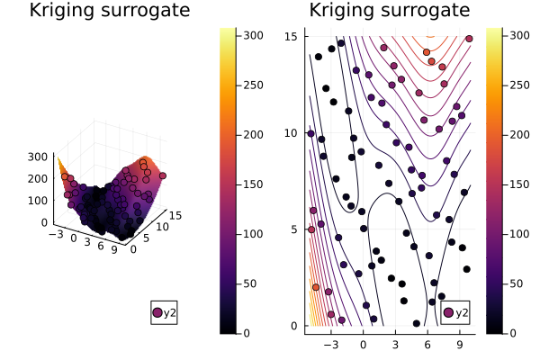

Increasing time_step raises the noise level; at large enough values the fit is dominated by the perturbation and the three basins of the original Branin function stop being recoverable from this many samples.