Mixture of Experts (MOE) Surrogate Tutorial

The Mixture of Experts (MOE) Surrogate model represents the interpolating function as a combination of other surrogate models. SurrogatesMOE is a Julia implementation of the Python version from the SMT project.

Surrogates.MOE — Type

MOE(x, y, expert_types; ndim = 1, n_clusters = 2, quantile = 10)

Mixture-of-experts surrogate backed by GaussianMixtures.jl.

This type is available when the GaussianMixtures extension is loaded. It clusters the input data, fits one local surrogate per cluster, and dispatches evaluation to the selected expert.

Fields

x: training inputs.
y: training responses.
c: fitted Gaussian-mixture clusters.
d: frozen distributions corresponding to the clusters.
m: fitted local surrogate models.
e: expert surrogate configurations.
nd: number of input dimensions.
nc: number of clusters.

Arguments

x: sample locations.
y: observed values at x.
expert_types: surrogate configurations used to build local experts.

Keywords

ndim: number of input dimensions.
n_clusters: number of mixture clusters.
quantile: quantile used when assigning local training data.

Returns

An MOE surrogate satisfying the generic surrogate interface.

source

MOE is most useful when we have a discontinuous function. For example, let's say we want to build a surrogate for the following function:

1D Example

function discont_1D(x)
    if x < 0.0
        return -5.0
    elseif x >= 0.0
        return 5.0
    end
end

discont_1D (generic function with 1 method)

Let's choose the MOE Surrogate for 1D. Note that we have to import the GaussianMixtures in addition to Surrogates and Plots.

using Surrogates
using GaussianMixtures
using Plots

lb = -1.0
ub = 1.0
x = sample(50, lb, ub, SobolSample())
y = discont_1D.(x)
scatter(
    x, y, label = "Sampled Points", xlims = (lb, ub), ylims = (-6.0, 7.0), legend = :top)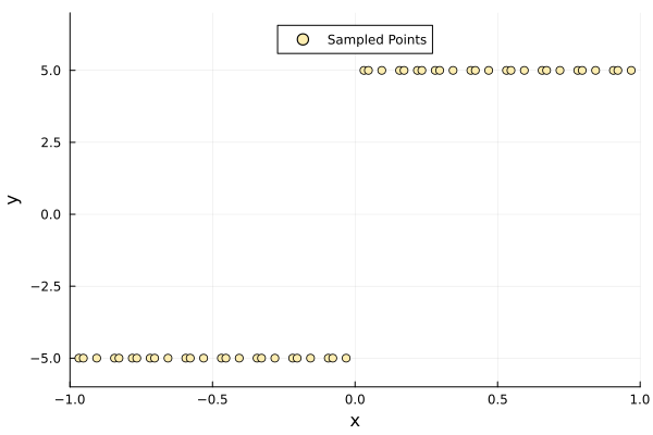

How does a regular surrogate perform on such a dataset?

RAD_1D = RadialBasis(x, y, lb, ub, rad = linearRadial(), scale_factor = 1.0, sparse = false)
RAD_at0 = RAD_1D(0.0) #true value should be 5.0

-7.050394859095663e-15

As we can see, the prediction is far from the ground truth. Now, how does the MOE perform?

expert_types = [
    RadialBasisStructure(radial_function = linearRadial(), scale_factor = 1.0,
        sparse = false),
    RadialBasisStructure(radial_function = linearRadial(), scale_factor = 1.0,
        sparse = false)
]

MOE_1D_RAD_RAD = MOE(x, y, expert_types)
MOE_at0 = MOE_1D_RAD_RAD(0.0)

5.5357142857142865

As we can see, the accuracy is significantly better.

Under the Hood: How SurrogatesMOE Works

First, we create Gaussian Mixture Models for the number of expert types provided using the x and y values. For example, in the above example, we create two clusters. Then, using a small test dataset kept aside from the input data, we choose the best surrogate model for each of the clusters. At prediction time, we use the appropriate surrogate model based on the cluster to which the new point belongs.

N-Dimensional Example

using Surrogates
using GaussianMixtures

# helper to test accuracy of predictors
function rmse(a, b)
    a = vec(a)
    b = vec(b)
    if (size(a) != size(b))
        println("error in inputs")
        return
    end
    n = size(a, 1)
    return sqrt(sum((a - b) .^ 2) / n)
end

# multidimensional input function
function discont_NDIM(x)
    if (x[1] >= 0.0 && x[2] >= 0.0)
        return sum(x .^ 2) + 5
    else
        return sum(x .^ 2) - 5
    end
end
lb = [-1.0, -1.0]
ub = [1.0, 1.0]
n = 150
x = sample(n, lb, ub, RandomSample())
y = discont_NDIM.(x)
x_test = sample(10, lb, ub, GoldenSample())

expert_types = [
    RadialBasisStructure(radial_function = linearRadial(), scale_factor = 1.0,
        sparse = false),
    RadialBasisStructure(radial_function = linearRadial(), scale_factor = 1.0,
        sparse = false)
]
moe_nd_rad_rad = MOE(x, y, expert_types, ndim = 2)
moe_pred_vals = moe_nd_rad_rad.(x_test)
true_vals = discont_NDIM.(x_test)
moe_rmse = rmse(true_vals, moe_pred_vals)
rbf = RadialBasis(x, y, lb, ub)
rbf_pred_vals = rbf.(x_test)
rbf_rmse = rmse(true_vals, rbf_pred_vals)
@show rbf_rmse, moe_rmse

(0.2521836501994461, 0.027416516025169622)

Usage Notes: Example With Other Surrogates

From the above example, simply change or add to the expert types:

using Surrogates
#To use Inverse Distance and Radial Basis Surrogates
expert_types = [
    KrigingStructure(p = [1.0, 1.0], theta = [1.0, 1.0]),
    InverseDistanceStructure(p = 1.0)
]

#With 3 Surrogates
expert_types = [
    RadialBasisStructure(radial_function = linearRadial(), scale_factor = 1.0,
        sparse = false),
    LinearStructure(),
    InverseDistanceStructure(p = 1.0)
]

3-element Vector{NamedTuple}:
 (name = "RadialBasis", radial_function = Surrogates.RadialFunction{Int64, Surrogates.var"#linearRadial##0#linearRadial##1"}(0, Surrogates.var"#linearRadial##0#linearRadial##1"()), scale_factor = 1.0, sparse = false)
 (name = "LinearSurrogate",)
 (name = "InverseDistanceSurrogate", p = 1.0)