Neural Network Surrogate Tutorial

It's possible to define a neural network as a surrogate, using Flux. This is useful because we can call optimization methods on it.

Surrogates.NeuralSurrogate — Type

NeuralSurrogate(x, y, lb, ub; model, loss, opt, n_epochs)

Neural-network surrogate backed by Flux.jl.

This type is available when the Flux extension is loaded. The fitted surrogate is callable as surrogate(x_new) and supports update! by retraining with appended observations.

Fields

x: training inputs.
y: training responses.
model: Flux model.
loss: training loss.
opt: optimizer state or optimizer object.
ps: vector of trainable model parameter arrays returned by Optimisers.trainables(model).
n_epochs: number of training epochs.
lb: lower bound of the input domain.
ub: upper bound of the input domain.

Arguments

x: sample locations.
y: observed values at x.
lb: lower bound of the input domain.
ub: upper bound of the input domain.

Keywords

model: Flux model used for prediction.
loss: loss function used during training.
opt: optimizer used during training.
n_epochs: number of training epochs.

Returns

A NeuralSurrogate satisfying the generic surrogate interface.

source

Surrogates.GENNSurrogate — Type

GENNSurrogate(x, y, dydx, lb, ub; model, opt, n_epochs, gamma,
    is_normalize = true)

Gradient-enhanced neural-network surrogate backed by Flux.jl.

This type is available when the Flux extension is loaded. It trains on both function observations and derivative observations. The fitted surrogate is callable as surrogate(x_new), supports predict_derivative, and can be updated with new samples.

Fields

x: training inputs.
y: training responses.
dydx: derivative observations stored as (n_outputs, n_inputs, n_samples).
model: Flux model.
opt: optimizer state or optimizer object.
ps: vector of trainable model parameter arrays returned by Optimisers.trainables(model).
n_epochs: number of training epochs.
lb: lower bound of the input domain.
ub: upper bound of the input domain.
gamma: derivative-loss weight.
x_mean: input normalization mean, or nothing.
x_std: input normalization scale, or nothing.
y_mean: output normalization mean, or nothing.
y_std: output normalization scale, or nothing.
is_normalize: whether normalization is enabled.

Arguments

x: sample locations.
y: observed values at x.
dydx: derivative observations.
lb: lower bound of the input domain.
ub: upper bound of the input domain.

Keywords

model: Flux model used for prediction.
opt: optimizer used during training.
n_epochs: number of training epochs.
gamma: derivative-loss weight.
is_normalize: whether to normalize inputs and outputs during training.

Returns

A GENNSurrogate satisfying the generic surrogate interface.

source

Surrogates.predict_derivative — Function

predict_derivative(genn::GENNSurrogate, x)

Evaluate the derivative predicted by a gradient-enhanced neural surrogate.

Arguments

genn::GENNSurrogate: fitted gradient-enhanced neural surrogate.
x: input location where the derivative should be predicted.

Returns

The derivative prediction at x, using the normalization convention stored in genn.

source

First of all we will define the Schaffer function we are going to build a surrogate for.

using Plots
default(c = :matter, legend = false, xlabel = "x", ylabel = "y")
using Surrogates
using Flux

function schaffer(x)
    x1 = x[1]
    x2 = x[2]
    fact1 = x1^2
    fact2 = x2^2
    y = fact1 + fact2
end

schaffer (generic function with 1 method)

Sampling

Let's define our bounds, this time we are working in two dimensions. In particular we want our first dimension x to have bounds 0, 8, and 0, 8 for the second dimension. We are taking 100 samples of the space using Sobol Sequences. We then evaluate our function on all the sampling points.

n_samples = 100
lower_bound = [0.0, 0.0]
upper_bound = [8.0, 8.0]

xys = sample(n_samples, lower_bound, upper_bound, SobolSample())
zs = schaffer.(xys)

100-element Vector{Float64}:
 10.1953125
 69.1953125
 39.6953125
 31.6953125
 10.1953125
 69.1953125
 31.6953125
 39.6953125
  5.6953125
 64.6953125
  ⋮
 46.064453125
  6.314453125
 64.314453125
 27.314453125
 47.814453125
  0.501953125
 40.501953125
 48.251953125
 48.751953125

xgrid = range(lower_bound[1], upper_bound[1], length = 100)
ygrid = range(lower_bound[2], upper_bound[2], length = 100)
p1 = surface(xgrid, ygrid, (x1, x2) -> schaffer((x1, x2)))
xs = [xy[1] for xy in xys]
ys = [xy[2] for xy in xys]
scatter!(xs, ys, zs)
p2 = contour(xgrid, ygrid, (x1, x2) -> schaffer((x1, x2)))
scatter!(xs, ys)
plot(p1, p2, title = "True function")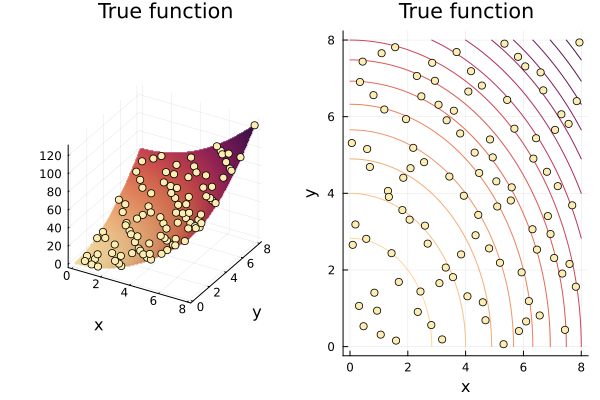

Building a surrogate

You can specify your own model, optimization function, loss functions, and epochs. As always, getting the model right is the hardest thing.

model1 = Chain(
    Dense(2, 32, relu),
    Dense(32, 32, relu),
    Dense(32, 1),
    first
)
neural = NeuralSurrogate(xys, zs, lower_bound, upper_bound, model = model1, n_epochs = 1000)

(::NeuralSurrogate{Matrix{Float64}, Matrix{Float64}, Flux.Chain{Tuple{Flux.Dense{typeof(NNlib.relu), Matrix{Float32}, Vector{Float32}}, Flux.Dense{typeof(NNlib.relu), Matrix{Float32}, Vector{Float32}}, Flux.Dense{typeof(identity), Matrix{Float32}, Vector{Float32}}, typeof(first)}}, typeof(Flux.Losses.mse), Optimisers.Adam{Float64, Tuple{Float64, Float64}, Float64}, Vector{AbstractArray}, Int64, Vector{Float64}, Vector{Float64}}) (generic function with 3 methods)

p1 = surface(xgrid, ygrid, (x, y) -> neural([x, y]))
scatter!(xs, ys, zs, marker_z = zs)
p2 = contour(xgrid, ygrid, (x, y) -> neural([x, y]))
scatter!(xs, ys, marker_z = zs)
plot(p1, p2, title = "Surrogate")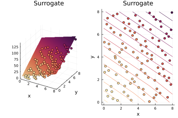

Optimization

We can now call an optimization function on the neural network:

surrogate_optimize!(schaffer, SRBF(), lower_bound, upper_bound, neural,
    SobolSample(), maxiters = 20, num_new_samples = 10)

(0.46875, 0.501953125)