Wendland Surrogate Tutorial

The Wendland surrogate uses a compactly supported radial kernel: a sample point influences predictions only within a finite radius of it. Most kernel pairs therefore contribute nothing, the interpolation matrix is sparse, and the surrogate allocates much less memory than a globally supported one. The coefficients are found with conjugate gradients; if that solve does not converge within maxiters, a warning is emitted and the fit should not be trusted.

Wendland(x, y, lb, ub; eps = 1.0, maxiters = 300, tol = 1.0e-6)

$f = x -> exp(-x^2)$

using Surrogates
using Plots

We sample f at 100 points between 0 and 1 using the sample function. The sampling points are chosen using a Sobol sequence, which is done by passing SobolSample() to sample.

n = 100
lower_bound = 0.0
upper_bound = 1.0
f = x -> exp(-x^2)
x = sample(n, lower_bound, upper_bound, SobolSample())
y = f.(x)

100-element Vector{Float64}:
 0.999450834440385
 0.7603420992361533
 0.5497973262437404
 0.9279586861644862
 0.8532075516884395
 0.4461099014964117
 0.6567372979278094
 0.9782072773172401
 0.956480737427535
 0.6032448395626249
 ⋮
 0.8397106792180511
 0.9177496036501366
 0.5332315942095883
 0.7446692912821248
 0.9981553899116735
 0.996572659247785
 0.7319617814344029
 0.5200533624689974
 0.9091637095195747

One dimension

Building a surrogate

eps is the reciprocal of the support radius: a sample point influences predictions within distance 1 / eps of it, and nowhere else. Here eps = 0.45 gives a radius of about 2.2, so every sample point reaches across the whole domain.

wend = Wendland(x, y, lower_bound, upper_bound, eps = 0.45)

(::Wendland{Vector{Float64}, Vector{Float64}, Float64, Float64, Vector{Float64}, Int64, Float64, Float64}) (generic function with 1 method)

plot(x, y, seriestype = :scatter, label = "Sampled points",
    xlims = (lower_bound, upper_bound), legend = :top)
plot!(f, label = "True function", xlims = (lower_bound, upper_bound), legend = :top)
plot!(wend, label = "Surrogate function", xlims = (lower_bound, upper_bound), legend = :top)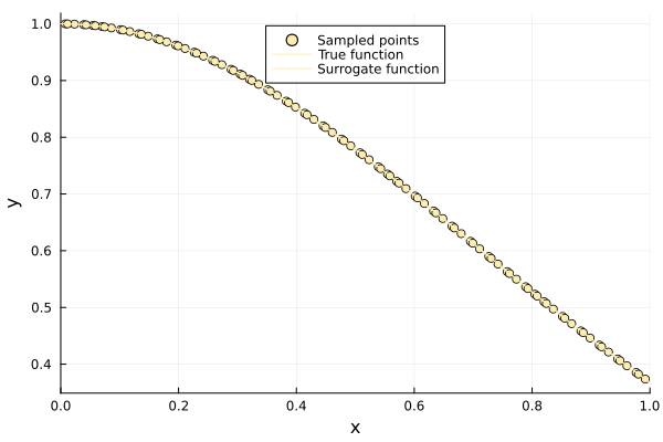

Choosing the support radius

Shrinking the support makes each prediction depend on fewer sample points. The surrogate still interpolates — it reproduces every sampled response whatever eps is — but between the samples it decays towards zero once the radius drops below the sample spacing:

grid = range(lower_bound, upper_bound, length = 400)
rms(v) = sqrt(sum(abs2, v) / length(v))

for eps in [0.45, 2.0, 20.0, 50.0]
    w = Wendland(x, y, lower_bound, upper_bound, eps = eps)
    println("eps = ", eps,
        "  radius = ", round(1 / eps, digits = 3),
        "  RMSE off the samples = ", round(rms([w(v) - f(v) for v in grid]), digits = 6),
        "  max error at the samples = ",
        round(maximum(abs(w(x[i]) - y[i]) for i in eachindex(x)), digits = 8))
end

eps = 0.45  radius = 2.222  RMSE off the samples = 2.0e-6  max error at the samples = 2.46e-6
eps = 2.0  radius = 0.5  RMSE off the samples = 9.4e-5  max error at the samples = 2.14e-6
eps = 20.0  radius = 0.05  RMSE off the samples = 0.008494  max error at the samples = 2.18e-6
eps = 50.0  radius = 0.02  RMSE off the samples = 0.055141  max error at the samples = 1.3e-7

plot(f, label = "True function", xlims = (lower_bound, upper_bound), legend = :top)
for eps in [0.45, 20.0, 50.0]
    w = Wendland(x, y, lower_bound, upper_bound, eps = eps)
    plot!(w, label = "eps = $eps", xlims = (lower_bound, upper_bound))
end
plot!()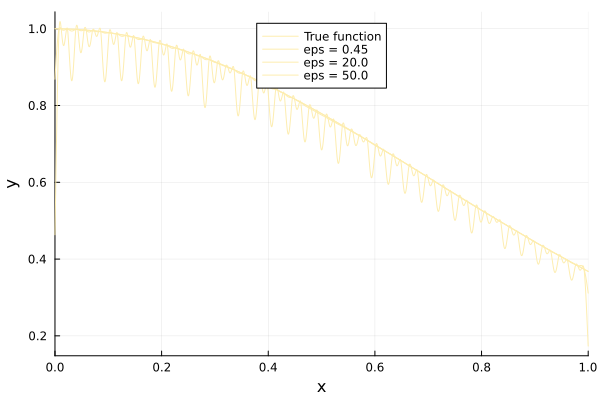

Several dimensions

The surrogate works the same way in more dimensions; only the bounds change shape. Note that the kernel exponent depends on the input dimension, so the same eps gives a slightly different profile.

using Surrogates
using Plots
default(c = :matter, legend = false, xlabel = "x", ylabel = "y")

function branin(x)
    x1, x2 = x[1], x[2]
    a, b, c, r, s, t = 1.0, 5.1 / (4 * pi^2), 5 / pi, 6.0, 10.0, 1 / (8 * pi)
    return a * (x2 - b * x1^2 + c * x1 - r)^2 + s * (1 - t) * cos(x1) + s
end

lower_bound = [-5.0, 0.0]
upper_bound = [10.0, 15.0]
xys = sample(200, lower_bound, upper_bound, SobolSample())
zs = branin.(xys);

200-element Vector{Float64}:
 148.0560267554004
  97.738872509658
  19.519858804218114
  15.334535299996283
  19.58430028520217
  85.33503631274715
  37.86282824541388
   7.016503458498236
  94.85700432033855
  60.76990376657528
   ⋮
  42.775586899193506
 217.38045214510993
  43.57743656698652
  35.711686855359176
  45.44560513224651
  21.76919408354652
 166.91843103721047
  15.128589307843406
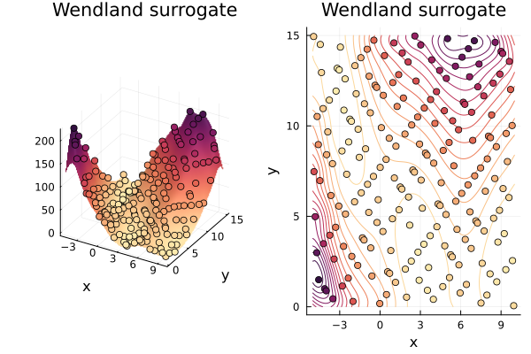
   1.49260763116982

The domain is about 15 units across, so a support radius of 5 (eps = 0.2) lets each sample point reach a useful neighbourhood without covering everything.

wend_ND = Wendland(xys, zs, lower_bound, upper_bound, eps = 0.2)
maximum(abs(wend_ND(xys[i]) - zs[i]) for i in eachindex(xys))

0.00015098172733729598

xs = [xy[1] for xy in xys]
ys = [xy[2] for xy in xys]
xgrid = range(lower_bound[1], upper_bound[1], length = 100)
ygrid = range(lower_bound[2], upper_bound[2], length = 100)
p1 = surface(xgrid, ygrid, (x, y) -> wend_ND([x y]))
scatter!(xs, ys, zs, marker_z = zs)
p2 = contour(xgrid, ygrid, (x, y) -> wend_ND([x y]))
scatter!(xs, ys, marker_z = zs)
plot(p1, p2, title = "Wendland surrogate")