Inverse distance surrogate tutorial

The Inverse Distance Surrogate (Shepard's method) is an interpolating method, and in this method, the unknown points are calculated with a weighted average of the sampling points. This model uses the inverse distance between the unknown and training points to predict the unknown point. We do not need to fit this model because the response of an unknown point x is computed with respect to the distance between x and the training points.

The single hyperparameter is the exponent p, which must be positive. Each sample point is weighted by 1 / distance^p, so a larger p concentrates the weight on the nearest samples and pushes the surrogate towards nearest-neighbour interpolation; a smaller p spreads the weight out and flattens the surrogate towards the mean of the responses. The prediction is a weighted average of the sampled responses, so it never leaves their range.

InverseDistanceSurrogate(x, y, lb, ub; p = 1.0)

using Surrogates

x = [0.0, 1.0, 2.0]
y = x .^ 2
surrogate = InverseDistanceSurrogate(x, y, 0.0, 2.0; p = 2.0)
surrogate(0.5)

Let's optimize the following function to use Inverse Distance Surrogate:

\[f(x) = sin(x) + sin(x)^2 + sin(x)^3\]

.

First of all, we have to import these two packages: Surrogates and Plots.

using Surrogates
using Plots

One dimension

Sampling

We choose to sample f in 100 points between 0 and 10 using the sample function. The sampling points are chosen using a Low Discrepancy, this can be done by passing HaltonSample() to the sample function.

f(x) = sin(x) + sin(x)^2 + sin(x)^3

n_samples = 100
lower_bound = 0.0
upper_bound = 10.0
x = sample(n_samples, lower_bound, upper_bound, HaltonSample())
y = f.(x)

scatter(x, y, label = "Sampled points", xlims = (lower_bound, upper_bound), legend = :top)
plot!(f, label = "True function", xlims = (lower_bound, upper_bound), legend = :top)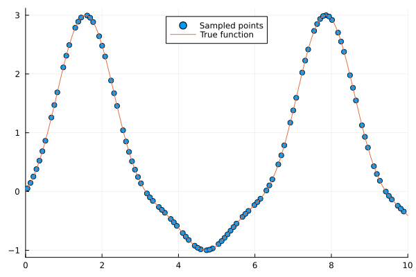

Building a Surrogate

InverseDistance = InverseDistanceSurrogate(x, y, lower_bound, upper_bound)
prediction = InverseDistance(5.0)

-0.310175502145857

Now, we will simply plot InverseDistance:

plot(x, y, seriestype = :scatter, label = "Sampled points",
    xlims = (lower_bound, upper_bound), legend = :top)
plot!(f, label = "True function", xlims = (lower_bound, upper_bound), legend = :top)
plot!(InverseDistance, label = "Surrogate function",
    xlims = (lower_bound, upper_bound), legend = :top)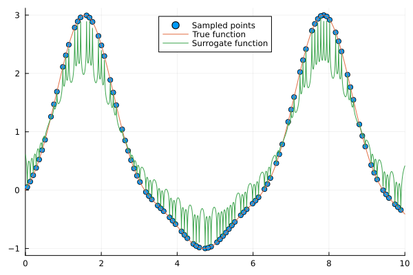

Choosing the exponent

The default p = 1.0 still gives distant samples enough weight to pull the surrogate towards the mean of the responses between the sampled points. Raising p concentrates the weight on the nearest samples:

plot(f, label = "True function", xlims = (lower_bound, upper_bound), legend = :top)
for p in [1.0, 2.0, 6.0]
    surr = InverseDistanceSurrogate(x, y, lower_bound, upper_bound, p = p)
    plot!(surr, label = "p = $p", xlims = (lower_bound, upper_bound))
end
plot!()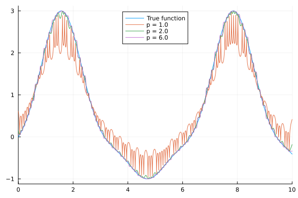

The flattening at p = 1 is easy to quantify. Away from the sampled points, compare how far the surrogate strays from the true function with how much of the function's own spread about the mean response it keeps:

grid = range(0.02, 9.98, length = 500)
ybar = sum(y) / length(y)
rms(v) = sqrt(sum(abs2, v) / length(v))

for p in [1.0, 2.0, 6.0]
    surr = InverseDistanceSurrogate(x, y, lower_bound, upper_bound, p = p)
    println("p = ", p,
        "  RMSE vs f = ", round(rms([surr(v) - f(v) for v in grid]), digits = 4),
        "  spread kept = ", round(rms([surr(v) - ybar for v in grid]), digits = 4))
end
println("f's own spread about ybar = ",
    round(rms([f(v) - ybar for v in grid]), digits = 4))

p = 1.0  RMSE vs f = 0.408  spread kept = 0.9275
p = 2.0  RMSE vs f = 0.0445  spread kept = 1.273
p = 6.0  RMSE vs f = 0.0443  spread kept = 1.2969
f's own spread about ybar = 1.2976

Whatever p is, the surrogate interpolates: at a sampled point it returns the sampled response exactly.

maximum(abs(InverseDistance(x[i]) - y[i]) for i in eachindex(x))

0.0

Optimizing

Having built a surrogate, we can now use it to search for minima in our original function f.

To optimize using our surrogate we call surrogate_optimize! method. We choose to use Stochastic RBF as the optimization technique and again Sobol sampling as the sampling technique.

surrogate_optimize!(
    f, SRBF(), lower_bound, upper_bound, InverseDistance, SobolSample())
scatter(x, y, label = "Sampled points", legend = :top)
plot!(f, label = "True function", xlims = (lower_bound, upper_bound), legend = :top)
plot!(InverseDistance, label = "Surrogate function",
    xlims = (lower_bound, upper_bound), legend = :top)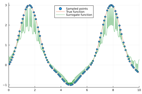

Several dimensions

First of all we will define the Schaffer function we are going to build a surrogate for. Notice, how its argument is a vector of numbers, one for each coordinate, and its output is a scalar.

using Plots
default(c = :matter, legend = false, xlabel = "x", ylabel = "y")
using Surrogates

function schaffer(x)
    x1 = x[1]
    x2 = x[2]
    fact1 = (sin(x1^2 - x2^2))^2 - 0.5
    fact2 = (1 + 0.001 * (x1^2 + x2^2))^2
    y = 0.5 + fact1 / fact2
end

schaffer (generic function with 1 method)

Sampling

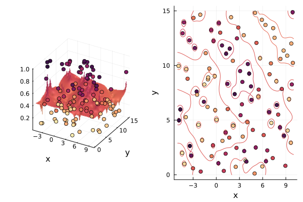
Let's define our bounds, this time we are working in two dimensions. In particular we want our first dimension x to have bounds -5, 10, and 0, 15 for the second dimension. We are taking 100 samples of the space using Sobol Sequences. We then evaluate our function on all the sampling points.

n_samples = 100
lower_bound = [-5.0, 0.0]
upper_bound = [10.0, 15.0]

xys = sample(n_samples, lower_bound, upper_bound, SobolSample())
zs = schaffer.(xys);

100-element Vector{Float64}:
 0.9466537351915296
 0.43907983917415927
 0.6244015434660956
 0.24029684484911762
 0.5445245406780457
 0.49603219937739446
 0.48167742985632134
 0.8026235934086707
 0.132320236918473
 0.12042018982244562
 ⋮
 0.8911120978015648
 0.3394437875244999
 0.36452094199290475
 0.6551197870142627
 0.6837172632966668
 0.09287469403688647
 0.7340338272751679
 0.06640336807634234
 0.6345377899252921

xgrid = range(lower_bound[1], upper_bound[1], length = 100)
ygrid = range(lower_bound[2], upper_bound[2], length = 100)
p1 = surface(xgrid, ygrid, (x1, x2) -> schaffer((x1, x2)))
xs = [xy[1] for xy in xys]
ys = [xy[2] for xy in xys]
scatter!(xs, ys, zs)
p2 = contour(xgrid, ygrid, (x1, x2) -> schaffer((x1, x2)))
scatter!(xs, ys)
plot(p1, p2, title = "True function")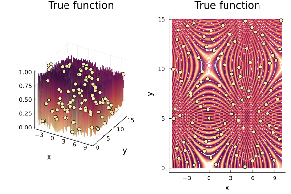

Building a Surrogate

Using the sampled points we build the surrogate, the steps are analogous to the 1-dimensional case.

InverseDistance = InverseDistanceSurrogate(xys, zs, lower_bound, upper_bound)

(::InverseDistanceSurrogate{Vector{Tuple{Float64, Float64}}, Vector{Float64}, Vector{Float64}, Vector{Float64}, Float64}) (generic function with 1 method)

p1 = surface(xgrid, ygrid, (x, y) -> InverseDistance([x y]))
scatter!(xs, ys, zs, marker_z = zs)
p2 = contour(xgrid, ygrid, (x, y) -> InverseDistance([x y]))
scatter!(xs, ys, marker_z = zs)
plot(p1, p2, title = "Surrogate")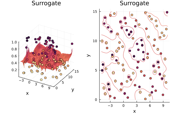

Optimizing

With our surrogate, we can now search for the minima of the function.

Notice how the new points sampled during the optimization process are added to the surrogate. The xys array we built it from is left untouched, so it is the surrogate's own sample list whose size changes.

length(xys), length(InverseDistance.x)

(100, 100)

surrogate_optimize!(schaffer, SRBF(), lower_bound, upper_bound,
    InverseDistance, SobolSample(), maxiters = 10)

((3.7890625, 1.2890625), 0.031658664860116315)

length(xys), length(InverseDistance.x)

(100, 110)

p1 = surface(xgrid, ygrid, (x, y) -> InverseDistance([x y]))
xs = [xy[1] for xy in InverseDistance.x]
ys = [xy[2] for xy in InverseDistance.x]
zs = schaffer.(InverseDistance.x)
scatter!(xs, ys, zs, marker_z = zs)
p2 = contour(xgrid, ygrid, (x, y) -> InverseDistance([x y]))
scatter!(xs, ys, marker_z = zs)
plot(p1, p2)