Rosenbrock function

The Rosenbrock function is defined as: $f(x) = \sum_{i=1}^{d-1}[ 100(x_{i+1}-x_i^2)^2 + (x_i - 1)^2]$

Its global minimum, $f(\mathbf{1}) = 0$, sits at the bottom of a narrow curved valley: easy to enter and hard to traverse, which is what the benchmark tests.

We treat the 2D version here, which is commonly written as: $f(x,y) = (1-x)^2 + 100(y-x^2)^2$ Let's import Surrogates and Plots:

using Surrogates
using PolyChaos
using Plots

Define the objective function:

function f(x)
    x1 = x[1]
    x2 = x[2]
    return (1 - x1)^2 + 100 * (x2 - x1^2)^2
end

f (generic function with 1 method)

Let's plot it:

n = 100
lb = [0.0, 0.0]
ub = [1.0, 1.0]
xys = sample(n, lb, ub, SobolSample())
zs = f.(xys);
xgrid = range(lb[1], ub[1], length = 100)
ygrid = range(lb[2], ub[2], length = 100)
p1 = surface(xgrid, ygrid, (x1, x2) -> f((x1, x2)))
xs = [xy[1] for xy in xys]
ys = [xy[2] for xy in xys]
scatter!(xs, ys, zs)
p2 = contour(xgrid, ygrid, (x1, x2) -> f((x1, x2)))
scatter!(xs, ys)
plot(p1, p2, title = "True function")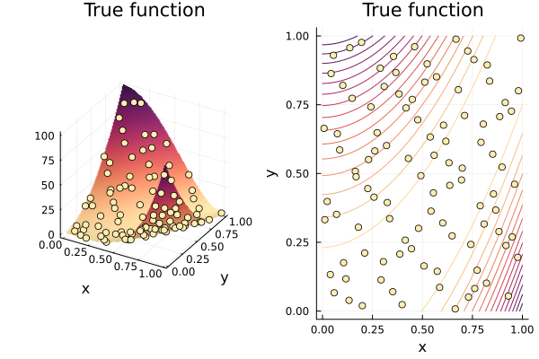

Fitting different surrogates:

mypoly = PolynomialChaosSurrogate(xys, zs, lb, ub)
loba = LobachevskySurrogate(xys, zs, lb, ub)
inver = InverseDistanceSurrogate(xys, zs, lb, ub)

(::InverseDistanceSurrogate{Vector{Tuple{Float64, Float64}}, Vector{Float64}, Vector{Float64}, Vector{Float64}, Float64}) (generic function with 1 method)

Plotting:

p1 = surface(xgrid, ygrid, (x, y) -> mypoly([x y]))
scatter!(xs, ys, zs, marker_z = zs)
p2 = contour(xgrid, ygrid, (x, y) -> mypoly([x y]))
scatter!(xs, ys, marker_z = zs)
plot(p1, p2, title = "Polynomial expansion")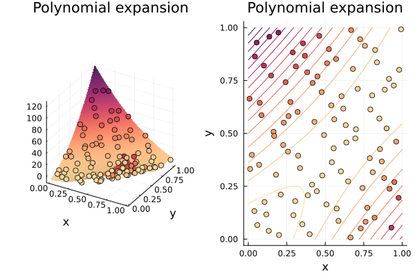

p1 = surface(xgrid, ygrid, (x, y) -> loba([x y]))
scatter!(xs, ys, zs, marker_z = zs)
p2 = contour(xgrid, ygrid, (x, y) -> loba([x y]))
scatter!(xs, ys, marker_z = zs)
plot(p1, p2, title = "Lobachevsky")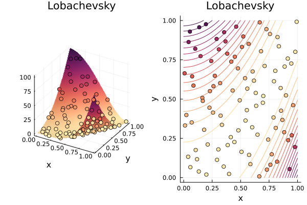

p1 = surface(xgrid, ygrid, (x, y) -> inver([x y]))
scatter!(xs, ys, zs, marker_z = zs)
p2 = contour(xgrid, ygrid, (x, y) -> inver([x y]))
scatter!(xs, ys, marker_z = zs)
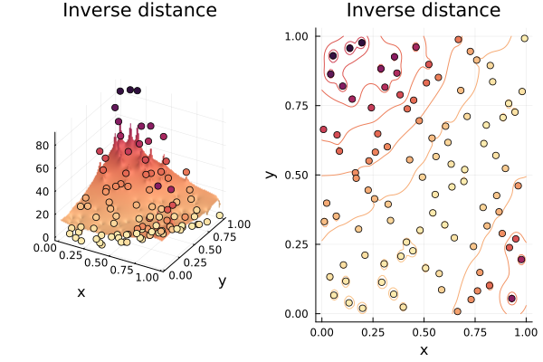
plot(p1, p2, title = "Inverse distance")