Cantilever Beam Function
The Cantilever Beam function is defined as: $f(t,w) = \frac{4L^3}{Ewt}\sqrt{ \left(\frac{Y}{t^2}\right)^2 + \left(\frac{X}{w^2}\right)^2 }$
with the input ordered as $x = (t, w)$ and the beam parameters $L$, $E$, $X$ and $Y$ fixed below. Note the $1/(wt)$ factor: the function is singular along $t = 0$ and $w = 0$, so it is evaluated on $[1, 8]^2$, away from both axes.
Let's import Surrogates and Plots:
using Surrogates
using PolyChaos
using Plots
Define the objective function:
function f(x)
    t = x[1]
    w = x[2]
    L = 100.0
    E = 2.770674127819261e7
    X = 530.8038576066307
    Y = 997.8714938733949
    return (4 * L^3) / (E * w * t) * sqrt((Y / t^2)^2 + (X / w^2)^2)
end
f (generic function with 1 method)Let's plot it:
n = 100
lb = [1.0, 1.0]
ub = [8.0, 8.0]
xys = sample(n, lb, ub, SobolSample())
zs = f.(xys)
xgrid = range(lb[1], ub[1], length = 100)
ygrid = range(lb[2], ub[2], length = 100)
p1 = surface(xgrid, ygrid, (x1, x2) -> f((x1, x2)))
xs = [xy[1] for xy in xys]
ys = [xy[2] for xy in xys]
scatter!(xs, ys, zs)
p2 = contour(xgrid, ygrid, (x1, x2) -> f((x1, x2)))
scatter!(xs, ys)
plot(p1, p2, title = "True function")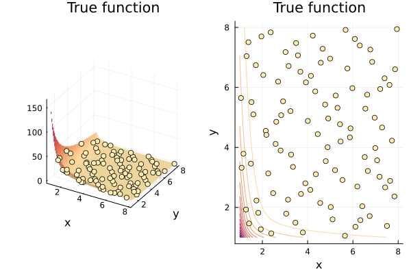
Fitting different surrogates:
mypoly = PolynomialChaosSurrogate(xys, zs, lb, ub)
loba = LobachevskySurrogate(xys, zs, lb, ub)
rad = RadialBasis(xys, zs, lb, ub)
(::RadialBasis{Surrogates.var"#linearRadial##0#linearRadial##1", Int64, Vector{Tuple{Float64, Float64}}, Vector{Float64}, Vector{Float64}, Vector{Float64}, LinearAlgebra.Transpose{Float64, Vector{Float64}}, Float64, Bool, Float64}) (generic function with 1 method)Plotting:
p1 = surface(xgrid, ygrid, (x1, x2) -> mypoly((x1, x2)))
scatter!(xs, ys, zs, marker_z = zs)
p2 = contour(xgrid, ygrid, (x1, x2) -> mypoly((x1, x2)))
scatter!(xs, ys, marker_z = zs)
plot(p1, p2, title = "Polynomial expansion")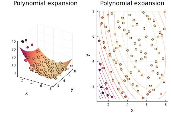
p1 = surface(xgrid, ygrid, (x1, x2) -> loba((x1, x2)))
scatter!(xs, ys, zs, marker_z = zs)
p2 = contour(xgrid, ygrid, (x1, x2) -> loba((x1, x2)))
scatter!(xs, ys, marker_z = zs)
plot(p1, p2, title = "Lobachevsky")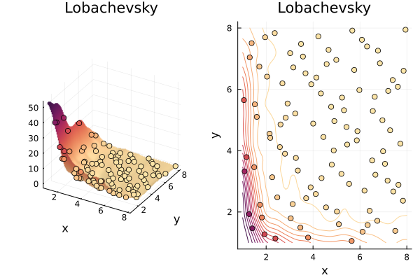
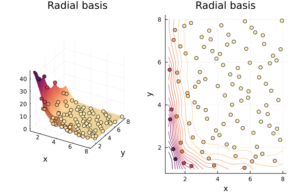
p1 = surface(xgrid, ygrid, (x1, x2) -> rad((x1, x2)))
scatter!(xs, ys, zs, marker_z = zs)
p2 = contour(xgrid, ygrid, (x1, x2) -> rad((x1, x2)))
scatter!(xs, ys, marker_z = zs)
plot(p1, p2, title = "Radial basis")