XGBoost Surrogate Tutorial

Gradient boosting fits an additive ensemble of decision trees, each round training a new tree on the residuals of the ensemble so far.

XGBoostSurrogate(x, y, lb, ub; num_round = 1)

We are going to use a xgboost surrogate to optimize $f(x)=sin(x)+sin(10/3 * x)$.

First of all import Surrogates, XGBoost and Plots.

using Surrogates
using XGBoost
using Plots

One dimension

Sampling

We choose to sample f in 100 points between 2.7 and 7.5 using the sample function. The sampling points are chosen using a Sobol sequence, this can be done by passing SobolSample() to the sample function.

f(x) = sin(x) + sin(10 / 3 * x)
n_samples = 100
lower_bound = 2.7
upper_bound = 7.5
x = sample(n_samples, lower_bound, upper_bound, SobolSample())
y = f.(x)
scatter(x, y, label = "Sampled points", xlims = (lower_bound, upper_bound))
plot!(f, label = "True function", xlims = (lower_bound, upper_bound), legend = :top)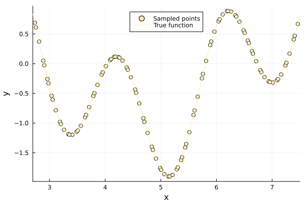

Building a surrogate

With our sampled points, we can build the XGBoost surrogate using the XGBoostSurrogate function.

xgboost_surrogate behaves like an ordinary function, which we can simply plot. Additionally, you can specify the number of boosting rounds using the parameter num_round

xgboost_surrogate = XGBoostSurrogate(
    x, y, lower_bound, upper_bound, num_round = 10)
plot(x, y, seriestype = :scatter, label = "Sampled points",
    xlims = (lower_bound, upper_bound), legend = :top)
plot!(f, label = "True function", xlims = (lower_bound, upper_bound), legend = :top)
plot!(xgboost_surrogate, label = "Surrogate function",
    xlims = (lower_bound, upper_bound), legend = :top)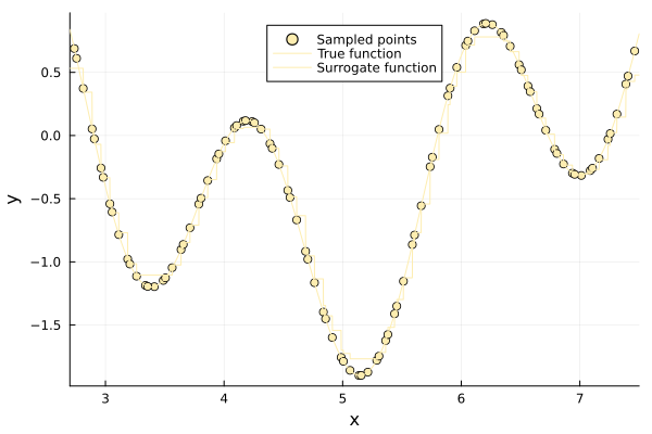

Optimizing

Having built a surrogate, we can now use it to search for minima in our original function f.

To optimize using our surrogate, we call surrogate_optimize! method. We choose to use Stochastic RBF as the optimization technique and again Sobol sampling as the sampling technique.

surrogate_optimize!(
    f, SRBF(), lower_bound, upper_bound, xgboost_surrogate, SobolSample())
scatter(x, y, label = "Sampled points")
plot!(f, label = "True function", xlims = (lower_bound, upper_bound), legend = :top)
plot!(xgboost_surrogate, label = "Surrogate function",
    xlims = (lower_bound, upper_bound), legend = :top)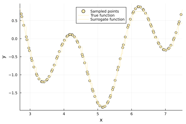

Several dimensions

First of all we will define the Bukin Function N. 6 function we are going to build a surrogate for.

using Plots
using Surrogates
using XGBoost

function bukin6(x)
    x1 = x[1]
    x2 = x[2]
    term1 = 100 * sqrt(abs(x2 - 0.01 * x1^2))
    term2 = 0.01 * abs(x1 + 10)
    y = term1 + term2
end

bukin6 (generic function with 1 method)

Sampling

Let's define our bounds, this time we are working in two dimensions. In particular we want our first dimension x to have bounds -5, 10, and 0, 15 for the second dimension. We are taking 100 samples of the space using Sobol Sequences. We then evaluate our function on all the sampling points.

n_samples = 100
lower_bound = [-5.0, 0.0]
upper_bound = [10.0, 15.0]

xys = sample(n_samples, lower_bound, upper_bound, SobolSample())
zs = bukin6.(xys)

100-element Vector{Float64}:
 240.06357349937196
 366.1237124935646
 133.98515572035174
 311.83595304317106
  58.59273381540032
 267.2623083319063
 197.07767387461334
 339.5519107340395
 177.00975695931635
 321.7658205306883
   ⋮
 332.649936145053
 130.3073403964058
 295.53097974529123
 231.43942144340937
 357.26111591015234
  90.95761265428854
 289.64930981289274
 206.03242446175668
 350.0208044124124

xgrid = range(lower_bound[1], upper_bound[1], length = 100)
ygrid = range(lower_bound[2], upper_bound[2], length = 100)
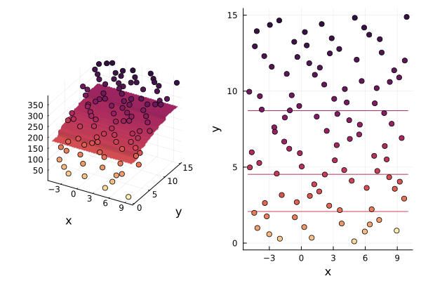
p1 = surface(xgrid, ygrid, (x1, x2) -> bukin6((x1, x2)))
xs = [xy[1] for xy in xys]
ys = [xy[2] for xy in xys]
scatter!(xs, ys, zs)
p2 = contour(xgrid, ygrid, (x1, x2) -> bukin6((x1, x2)))
scatter!(xs, ys)
plot(p1, p2, title = "True function")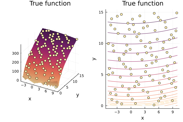

Building a surrogate

Using the sampled points, we build the surrogate, the steps are analogous to the 1-dimensional case.

XGBoost = XGBoostSurrogate(xys, zs, lower_bound, upper_bound)

(::XGBoostSurrogate{Matrix{Float64}, Vector{Float64}, XGBoost.Booster, Vector{Float64}, Vector{Float64}, Int64}) (generic function with 2 methods)

p1 = surface(xgrid, ygrid, (x, y) -> XGBoost([x y]))
scatter!(xs, ys, zs, marker_z = zs)
p2 = contour(xgrid, ygrid, (x, y) -> XGBoost([x y]))
scatter!(xs, ys, marker_z = zs)
plot(p1, p2, title = "Surrogate")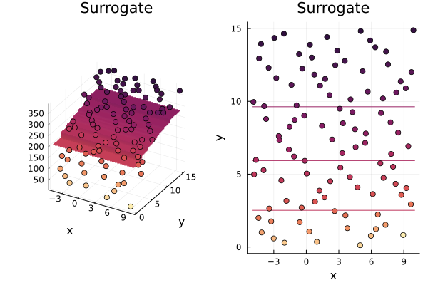

Optimizing

With our surrogate, we can now search for the minima of the function.

Notice how the new sampled points, which were created during the optimization process, are appended to the xys array. This is why its size changes.

size(xys)

(100,)

surrogate_optimize!(
    bukin6, SRBF(), lower_bound, upper_bound, XGBoost, SobolSample(), maxiters = 20)

(8.9453125, 14.376187341667872)

size(xys)

(100,)

p1 = surface(xgrid, ygrid, (x, y) -> XGBoost([x y]))
xs = [xy[1] for xy in xys]
ys = [xy[2] for xy in xys]
zs = bukin6.(xys)
scatter!(xs, ys, zs, marker_z = zs)
p2 = contour(xgrid, ygrid, (x, y) -> XGBoost([x y]))
scatter!(xs, ys, marker_z = zs)
plot(p1, p2)