Polynomial Chaos Surrogate Tutorial
We can create a surrogate using a polynomial expansion, with a different polynomial basis depending on the distribution of the data we are trying to fit. Under the hood, PolyChaos.jl has been used. It is possible to specify a type of polynomial for each dimension of the problem.
Surrogates.PolynomialChaosSurrogate — Type
PolynomialChaosSurrogate(x, y, lb, ub; orthopolys)Polynomial-chaos surrogate backed by PolyChaos.jl.
This type is available when the PolyChaos extension is loaded. It fits polynomial-chaos coefficients and evaluates the resulting expansion through the generic surrogate call interface.
Fields
x: training inputs.y: training responses.lb: lower bound of the input domain.ub: upper bound of the input domain.coeff: fitted polynomial-chaos coefficients.orthopolys: orthogonal-polynomial basis.num_of_multi_indexes: number of multi-index terms in the expansion.
Arguments
x: sample locations.y: observed values atx.lb: lower bound of the input domain.ub: upper bound of the input domain.
Returns
A PolynomialChaosSurrogate satisfying the generic surrogate interface.
Sampling
We choose to sample f in 100 points between 1 and 6 using the sample function. The sampling points are chosen from a low-discrepancy sequence, by passing HaltonSample() to the sample function.
using Surrogates
using PolyChaos
using Plots

n = 100
lower_bound = 1.0
upper_bound = 6.0
x = sample(n, lower_bound, upper_bound, HaltonSample())
f = x -> log(x) * x + sin(x)
y = f.(x)
scatter(x, y, label = "Sampled points", xlims = (lower_bound, upper_bound), legend = :top)
plot!(f, label = "True function", xlims = (lower_bound, upper_bound), legend = :top)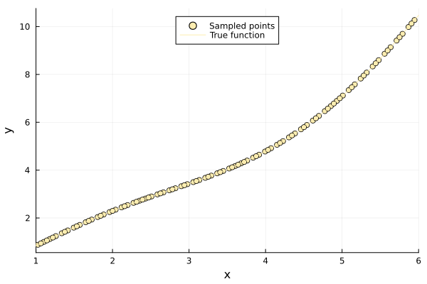
Building a Surrogate
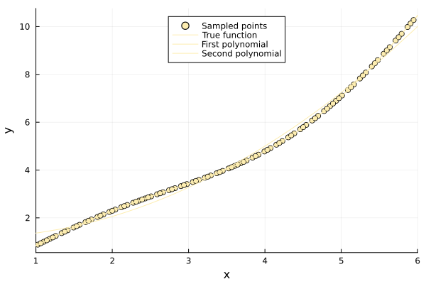
poly1 = PolynomialChaosSurrogate(x, y, lower_bound, upper_bound)
poly2 = PolynomialChaosSurrogate(
    x, y, lower_bound, upper_bound, orthopolys = GaussOrthoPoly(5))
plot(x, y, seriestype = :scatter, label = "Sampled points",
    xlims = (lower_bound, upper_bound), legend = :top)
plot!(f, label = "True function", xlims = (lower_bound, upper_bound), legend = :top)
plot!(poly1, label = "First polynomial", xlims = (lower_bound, upper_bound), legend = :top)
plot!(poly2, label = "Second polynomial", xlims = (lower_bound, upper_bound), legend = :top)