Gaussian Process Surrogate Tutorial

Gaussian Process regression in Surrogates.jl is implemented as a simple wrapper around the AbstractGPs.jl package. AbstractGPs comes with a variety of covariance functions (kernels). See KernelFunctions.jl for examples.

Surrogates.AbstractGPSurrogate — Type

AbstractGPSurrogate(x, y; gp = GP(Matern52Kernel()), Σy = 0.1)

Gaussian-process surrogate backed by AbstractGPs.jl.

This type is available when the AbstractGPs extension is loaded. It is a stochastic surrogate: surrogate(x) evaluates the posterior mean, and std_error_at_point returns the posterior standard deviation.

Fields

x: training inputs.
y: training responses.
gp: prior Gaussian process.
gp_posterior: posterior process fitted to x and y.
Σy: observation-noise covariance or scale.

Arguments

x: sample locations.
y: observed values at x.

Keywords

gp: AbstractGPs prior process.
Σy: observation noise passed to the finite GP posterior.

Returns

An AbstractGPSurrogate satisfying the stochastic surrogate interface.

source

Surrogates.logpdf_surrogate — Function

logpdf_surrogate(surrogate)

Return the log marginal likelihood or log density associated with a stochastic surrogate.

Arguments

surrogate: stochastic surrogate implementation.

Returns

A scalar log-density value. Methods are supplied by extensions that can compute the value for their backing model.

source

Tip

The examples below demonstrate the use of AbstractGPs with out-of-the-box settings without hyperparameter optimization (i.e. without changing parameters like lengthscale, signal variance, and noise variance). Beyond hyperparameter optimization, careful initialization of hyperparameters and priors on the parameters is required for this surrogate to work properly. For more details on how to fit GPs in practice, check out A Practical Guide to Gaussian Processes.

Also see this example to understand hyperparameter optimization with AbstractGPs.

1D Example

In the example below, the 'gp_surrogate' assignment code can be commented / uncommented to see how the different kernels influence the predictions.

using Surrogates
using Plots
using AbstractGPs

f(x) = (6 * x - 2)^2 * sin(12 * x - 4)
n_samples = 100
lower_bound = 0.0
upper_bound = 1.0
xs = lower_bound:0.001:upper_bound
x = sample(n_samples, lower_bound, upper_bound, SobolSample())
y = f.(x)

gp_surrogate = AbstractGPSurrogate(
    x, y, gp = GP(PolynomialKernel(; c = 2.0, degree = 15)), Σy = 0.25)
plot(x, y, seriestype = :scatter, label = "Sampled points",
    xlims = (lower_bound, upper_bound), ylims = (-7, 17), legend = :top)
plot!(xs, f.(xs), label = "True function", legend = :top)
plot!(0:0.001:1, gp_surrogate.gp_posterior; label = "Posterior", ribbon_scale = 2)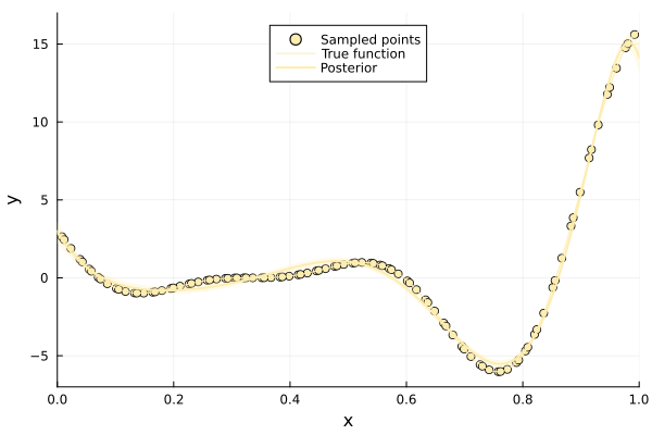

Optimization Example

This example shows the use of AbstractGP Surrogates to find the minima of a function:

using Surrogates
using Plots
using AbstractGPs

f(x) = (x - 2)^2
n_samples = 100
lower_bound = 0.0
upper_bound = 4.0
xs = lower_bound:0.1:upper_bound
x = sample(n_samples, lower_bound, upper_bound, SobolSample())
y = f.(x)
gp_surrogate = AbstractGPSurrogate(x, y)
surrogate_optimize!(f, SRBF(), lower_bound, upper_bound, gp_surrogate, SobolSample())

(2.0006250000000003, 3.9062500000039966e-7)

Plotting the function and the sampled points:

scatter(gp_surrogate.x, gp_surrogate.y, label = "Sampled points",
    ylims = (-1.0, 5.0), legend = :top)
plot!(xs, gp_surrogate.(xs), label = "Surrogate function",
    ribbon = p -> Surrogates.std_error_at_point(gp_surrogate, p), legend = :top)
plot!(xs, f.(xs), label = "True function", legend = :top)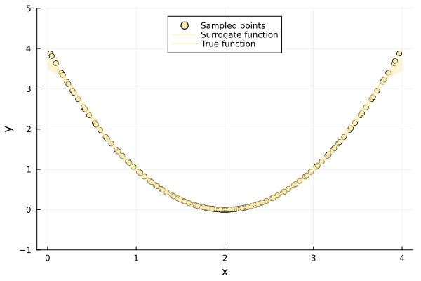

ND Example

using Plots
default(c = :matter, legend = false, xlabel = "x", ylabel = "y")
using Surrogates
using AbstractGPs

hypot_func = z -> 3 * hypot(z...) + 1
n_samples = 100
lower_bound = [-1.0, -1.0]
upper_bound = [1.0, 1.0]

xys = sample(n_samples, lower_bound, upper_bound, SobolSample())
zs = hypot_func.(xys)

xgrid = range(lower_bound[1], upper_bound[1], length = 100)
ygrid = range(lower_bound[2], upper_bound[2], length = 100)
p1 = surface(xgrid, ygrid, (x1, x2) -> hypot_func((x1, x2)))
xs = [xy[1] for xy in xys]
ys = [xy[2] for xy in xys]
scatter!(xs, ys, zs)
p2 = contour(xgrid, ygrid, (x1, x2) -> hypot_func((x1, x2)))
scatter!(xs, ys)
plot(p1, p2, title = "True function")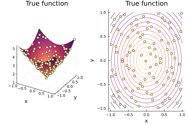

Now let's see how our surrogate performs:

gp_surrogate = AbstractGPSurrogate(xys, zs)
p1 = surface(xgrid, ygrid, (x, y) -> gp_surrogate([x y]))
scatter!(xs, ys, zs, marker_z = zs)
p2 = contour(xgrid, ygrid, (x, y) -> gp_surrogate([x y]))
scatter!(xs, ys, marker_z = zs)
plot(p1, p2, title = "Surrogate")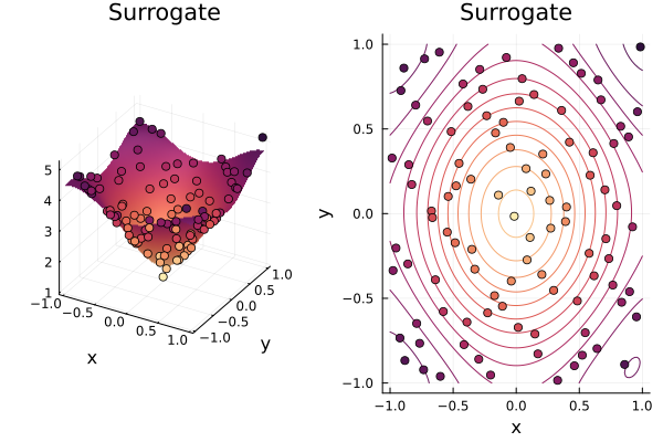

gp_surrogate((0.2, 0.2))

1.848078202411515

hypot_func((0.2, 0.2))

1.8485281374238571

And this is our log marginal posterior predictive probability:

logpdf_surrogate(gp_surrogate)

137.64470288774618