Lobachevsky Surrogate Tutorial

Lobachevsky splines function is a function that is used for univariate and multivariate scattered interpolation. Introduced by Lobachevsky in 1842 to investigate errors in astronomical measurements.

The surrogate has two hyperparameters. alpha is the kernel scale and must lie in (0, 4], one value per input dimension in the multivariate case; a scale of zero would make every kernel value identical and the interpolation system singular. n is the kernel order and must be even, positive and at most 20, since the kernel evaluates factorial(n).

Unlike the other surrogates here, a Lobachevsky spline has a closed-form integral, and one coordinate can be integrated out to leave a surrogate on the remaining ones.

lobachevsky_integrate_dimension(loba::LobachevskySurrogate, lb, ub, dim)

We are going to use a Lobachevsky surrogate to optimize $f(x)=sin(x)+sin(10/3 * x)$.

First of all import Surrogates and Plots.

using Surrogates
using Plots

One dimension

Sampling

We choose to sample f in 100 points between 1 and 4 using the sample function. The sampling points are chosen using a Sobol sequence, this can be done by passing SobolSample() to the sample function.

f(x) = sin(x) + sin(10 / 3 * x)
n_samples = 100
lower_bound = 1.0
upper_bound = 4.0
x = sample(n_samples, lower_bound, upper_bound, SobolSample())
y = f.(x)
scatter(x, y, label = "Sampled points", xlims = (lower_bound, upper_bound))
plot!(f, label = "True function", xlims = (lower_bound, upper_bound))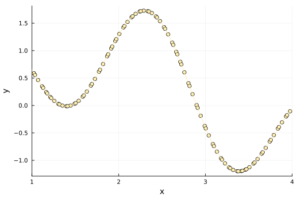

Building a surrogate

With our sampled points, we can build the Lobachevsky surrogate using the LobachevskySurrogate function.

lobachevsky_surrogate behaves like an ordinary function, which we can simply plot. alpha sets the kernel scale and n its order; a larger n makes the kernel approach a Gaussian radial basis function.

alpha = 2.0
n = 6
lobachevsky_surrogate = LobachevskySurrogate(
    x, y, lower_bound, upper_bound, alpha = 2.0, n = 6)
plot(x, y, seriestype = :scatter, label = "Sampled points",
    xlims = (lower_bound, upper_bound), legend = true)
plot!(f, label = "True function", xlims = (lower_bound, upper_bound))
plot!(
    lobachevsky_surrogate, label = "Surrogate function", xlims = (lower_bound, upper_bound))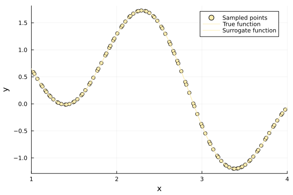

Optimizing

Having built a surrogate, we can now use it to search for minima in our original function f.

To optimize using our surrogate we call surrogate_optimize! method. We choose to use Stochastic RBF as the optimization technique and again Sobol sampling as the sampling technique.

surrogate_optimize!(
    f, SRBF(), lower_bound, upper_bound, lobachevsky_surrogate, SobolSample())
scatter(x, y, label = "Sampled points")
plot!(f, label = "True function", xlims = (lower_bound, upper_bound))
plot!(
    lobachevsky_surrogate, label = "Surrogate function", xlims = (lower_bound, upper_bound))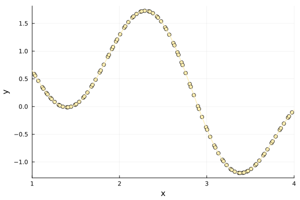

The closed-form integral

The Lobachevsky spline integrates in closed form, which the other surrogates in this package do not. lobachevsky_integral evaluates that formula, and it agrees with numerical integration of the same surrogate to round-off:

using QuadGK

closed = lobachevsky_integral(lobachevsky_surrogate, lower_bound, upper_bound)
numerical = quadgk(lobachevsky_surrogate, lower_bound, upper_bound)[1]
truth = quadgk(f, lower_bound, upper_bound)[1]

println("closed form            = ", closed)
println("quadrature of surrogate= ", numerical)
println("quadrature of f        = ", truth)
println("relative difference    = ", abs(closed - numerical) / abs(numerical))

closed form            = 0.6834380553917114
quadrature of surrogate= 0.6834380518277899
quadrature of f        = 0.683437211321203
relative difference    = 5.2146957309810685e-9

In the example below, it shows how to use lobachevsky_surrogate for higher dimension problems.

Several dimensions

First of all, we will define the Schaffer function we are going to build surrogate for. Notice, one how its argument is a vector of numbers, one for each coordinate, and its output is a scalar.

using Plots
default(c = :matter, legend = false, xlabel = "x", ylabel = "y")
using Surrogates

function schaffer(x)
    x1 = x[1]
    x2 = x[2]
    fact1 = x1^2
    fact2 = x2^2
    y = fact1 + fact2
end

schaffer (generic function with 1 method)

Sampling

Let's define our bounds, this time we are working in two dimensions. In particular, we want our first dimension x to have bounds 0, 8, and 0, 8 for the second dimension. We are taking 60 samples of the space using Sobol Sequences. We then evaluate our function on all of the sampling points.

n_samples = 60
lower_bound = [0.0, 0.0]
upper_bound = [8.0, 8.0]

xys = sample(n_samples, lower_bound, upper_bound, SobolSample())
zs = schaffer.(xys);

60-element Vector{Float64}:
   4.65625
  56.65625
  40.65625
  22.65625
  12.65625
  80.65625
  38.65625
  52.65625
   3.90625
  55.90625
   ⋮
  56.7578125
  31.0078125
 126.0078125
  39.0078125
  39.0078125
   8.0078125
  71.0078125
  55.5078125
  31.5078125

xgrid = range(lower_bound[1], upper_bound[1], length = 100)
ygrid = range(lower_bound[2], upper_bound[2], length = 100)
p1 = surface(xgrid, ygrid, (x1, x2) -> schaffer((x1, x2)))
xs = [xy[1] for xy in xys]
ys = [xy[2] for xy in xys]
scatter!(xs, ys, zs)
p2 = contour(xgrid, ygrid, (x1, x2) -> schaffer((x1, x2)))
scatter!(xs, ys)
plot(p1, p2, title = "True function")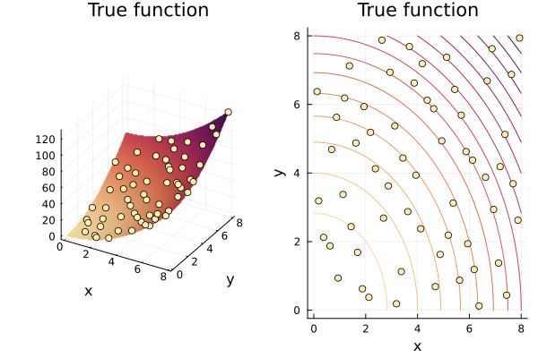

Building a surrogate

Using the sampled points, we build the surrogate, the steps are analogous to the 1-dimensional case.

Lobachevsky = LobachevskySurrogate(
    xys, zs, lower_bound, upper_bound, alpha = [2.4, 2.4], n = 8)

(::LobachevskySurrogate{Vector{Tuple{Float64, Float64}}, Vector{Float64}, Vector{Float64}, Int64, Vector{Float64}, Vector{Float64}, Vector{Float64}, Bool}) (generic function with 2 methods)

p1 = surface(xgrid, ygrid, (x, y) -> Lobachevsky([x y]))
scatter!(xs, ys, zs, marker_z = zs)
p2 = contour(xgrid, ygrid, (x, y) -> Lobachevsky([x y]))
scatter!(xs, ys, marker_z = zs)
plot(p1, p2, title = "Surrogate")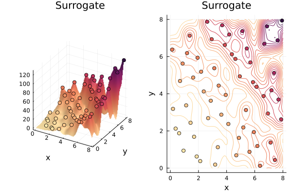

Optimizing

With our surrogate, we can now search for the minima of the function.

The points sampled during the optimization process are added to the surrogate. The xys array we built it from is left untouched, so it is the surrogate's own sample list whose size changes.

length(xys), length(Lobachevsky.x)

(60, 60)

surrogate_optimize!(schaffer, SRBF(), lower_bound, upper_bound, Lobachevsky,
    SobolSample(), maxiters = 1, num_new_samples = 10)

((0.9375, 0.9375), 1.7578125)

length(xys), length(Lobachevsky.x)

(60, 61)

p1 = surface(xgrid, ygrid, (x, y) -> Lobachevsky([x y]))
xys = Lobachevsky.x
xs = [i[1] for i in xys]
ys = [i[2] for i in xys]
zs = schaffer.(xys)
scatter!(xs, ys, zs, marker_z = zs)
p2 = contour(xgrid, ygrid, (x, y) -> Lobachevsky([x y]))
scatter!(xs, ys, marker_z = zs)
plot(p1, p2)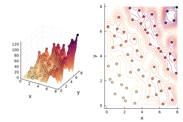

Integrating out a coordinate

lobachevsky_integrate_dimension integrates the surrogate over one coordinate and returns a surrogate on the remaining ones — the marginal. Here we integrate the second coordinate of the two-dimensional model over [0, 8], leaving a one-dimensional surrogate in x1:

using QuadGK

marginal = lobachevsky_integrate_dimension(
    Lobachevsky, lower_bound, upper_bound, 2)

for x1 in [1.0, 3.0, 6.0]
    direct = quadgk(t -> Lobachevsky((x1, t)), lower_bound[2], upper_bound[2])[1]
    println("x1 = ", x1, "  marginal = ", marginal(x1), "  quadrature = ", direct)
end

x1 = 1.0  marginal = 130.30498194113963  quadrature = 130.30498194299375
x1 = 3.0  marginal = 204.6338622464863  quadrature = 204.63386223115214
x1 = 6.0  marginal = 284.90997666261006  quadrature = 284.9099765802839

Integrating that marginal over the remaining coordinate gives the same answer as integrating the two-dimensional surrogate over the whole box:

lobachevsky_integral(marginal, marginal.lb, marginal.ub),
lobachevsky_integral(Lobachevsky, lower_bound, upper_bound)

(1980.4629474080182, 1980.4629474080184)

Vector-valued responses

The interpolant is linear in the responses and the kernel matrix does not involve them, so several outputs can be fitted at once against the same matrix. Pass a vector of equal-length response vectors and the surrogate returns a vector:

using Surrogates

f = x -> [sin(x), cos(x), 2x]
x = sample(20, 0.0, 4.0, SobolSample())
y = f.(x)

multi = LobachevskySurrogate(x, y, 0.0, 4.0, alpha = 2.0, n = 6)
multi(1.3)

3-element Vector{Float64}:
 0.9636618357959463
 0.26745277376766374
 2.5997336510399833

Each output is the surrogate that would have been fitted to that output alone, so lobachevsky_integral and lobachevsky_integrate_dimension return one value per output as well:

lobachevsky_integral(multi, 0.0, 4.0)

3-element Vector{Float64}:
  1.6544788766426635
 -0.7571590001710113
 15.995950070846462