Second Order Polynomial Surrogate Tutorial

The second-order polynomial model is the least-squares fit

$y = Xβ + ϵ$

where $X$ is the design matrix of the linear model augmented with the $d(d-1)/2$ pairwise products of the variables and their $d$ squares, for $1 + 2d + d(d-1)/2$ columns in all. Because it is a regression rather than an interpolation, the surrogate does not pass through the samples once there are more of them than coefficients; what it guarantees instead is that the residual is orthogonal to every column of $X$.

That column count is also the minimum number of samples: fewer leave the quadratic underdetermined, and so do degenerate designs such as collinear points, both of which are rejected rather than silently fitted.

Surrogates.SecondOrderPolynomialSurrogate — Type

SecondOrderPolynomialSurrogate(x, y, lb, ub)

Fit a full second-order polynomial to (x, y) by least squares.

For d-dimensional inputs the model is the complete quadratic

\[\hat f(p) = \beta_0 + \sum_{j=1}^{d} \beta_j p_j + \sum_{j<k} \beta_{jk} p_j p_k + \sum_{j=1}^{d} \beta_{jj} p_j^2\]

with 1 + 2d + d(d - 1) ÷ 2 coefficients. It is a regression surrogate, not an interpolant: with more samples than coefficients it does not pass through the data, and the residual is orthogonal to every column of the design matrix.

Fields

x: sampled input points.
y: scalar or vector responses corresponding to x.
β: fitted coefficients, ordered as described under Coefficient order.
lb: lower bound of the modeled domain.
ub: upper bound of the modeled domain.

Arguments

x: training points, as numbers for one-dimensional inputs or as equal-length tuples or vectors otherwise. At least 1 + 2d + d(d - 1) ÷ 2 points are required; fewer throws an ArgumentError. The count is necessary but not sufficient: a degenerate design (points collinear in two dimensions, say) leaves the quadratic unidentifiable and is rejected with an ArgumentError too, rather than silently returning one of its infinitely many minimum-norm fits.
y: training responses, one per point. Numbers give a scalar surrogate; equal-length vectors or tuples give a multi-output one, fitted one output per column against a single shared factorization.
lb: lower domain bound.
ub: upper domain bound matching lb.

Returns

A callable SecondOrderPolynomialSurrogate supporting update!(surrogate, x_new, y_new), which refits the coefficients after adding observations.

Coefficient order

β follows the columns of the design matrix: the intercept, then each coordinate, then the pairwise products in lexicographic order, then the squares. In two dimensions that is

β = [1, p₁, p₂, p₁p₂, p₁², p₂²]

so a target written in matrix form, a + bᵀp + pᵀCp with symmetric C, has β = [a, b₁, b₂, 2C₁₂, C₁₁, C₂₂] — the cross coefficient is 2C₁₂, since C contributes the off-diagonal term twice.

For vector responses β is a matrix with one column per output, and evaluation returns a vector.

Element types

The fit is carried out in float(eltype) of the samples, so Float32 and BigFloat inputs keep their precision and integer or rational inputs are promoted the same way \ would promote them. Queries may be given in any type that promotes against the fit.

Differentiability

Evaluation is differentiable in the query point with both ForwardDiff and Zygote — gradients, Hessians, multi-output Jacobians, and nested duals. The fit is differentiable in the training data with ForwardDiff, which is how to obtain sensitivities of a fitted value to the samples it was built from; Zygote cannot trace the fit, as the design matrix is built by mutation.

Example

using Surrogates

x = [(0.0,), (1.0,), (2.0,)]
y = [0.0, 1.0, 4.0]
surrogate = SecondOrderPolynomialSurrogate(x, y, [0.0], [2.0])
surrogate((1.5,))

source

using Surrogates
using Plots

Sampling

f = x -> 3 * sin(x) + 10 / x
lb = 3.0
ub = 6.0
n = 100
x = sample(n, lb, ub, HaltonSample())
y = f.(x)
scatter(x, y, label = "Sampled points", xlims = (lb, ub))
plot!(f, label = "True function", xlims = (lb, ub))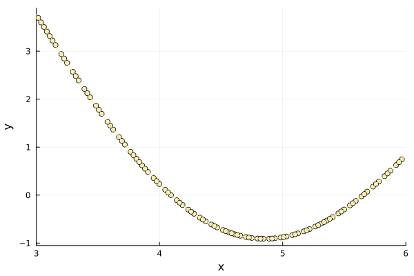

Building the surrogate

sec = SecondOrderPolynomialSurrogate(x, y, lb, ub)
plot(x, y, seriestype = :scatter, label = "Sampled points", xlims = (lb, ub))
plot!(f, label = "True function", xlims = (lb, ub))
plot!(sec, label = "Surrogate function", xlims = (lb, ub))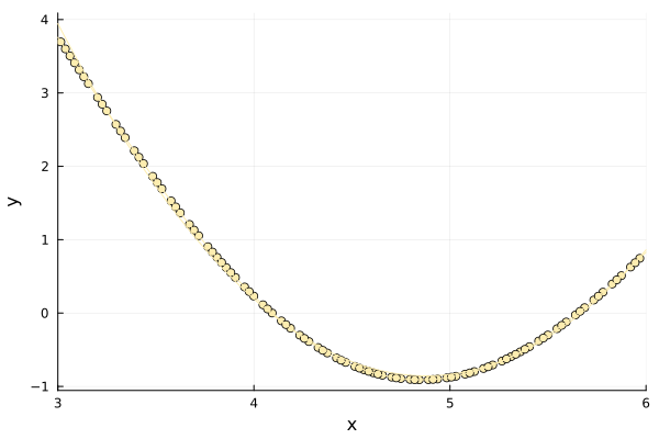

Optimizing

surrogate_optimize!(f, SRBF(), lb, ub, sec, SobolSample())
scatter(x, y, label = "Sampled points")
plot!(f, label = "True function", xlims = (lb, ub))
plot!(sec, label = "Surrogate function", xlims = (lb, ub))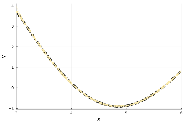

The optimization method successfully found the minimum.

Multi-output responses

Passing a vector response per sample fits one column of coefficients per output against a single shared factorization, and evaluation returns a vector.

using Surrogates

lb = [0.0, 0.0]
ub = [10.0, 10.0]
f = p -> [p[1]^2, p[1] * p[2]]
x = sample(30, lb, ub, SobolSample())
y = f.(x)
sec = SecondOrderPolynomialSurrogate(x, y, lb, ub)
sec((2.0, 3.0))

2-element Vector{Float64}:
 4.000000000000003
 5.999999999999995

Both outputs are exactly quadratic, so they are recovered to round-off:

f((2.0, 3.0))

2-element Vector{Float64}:
 4.0
 6.0

Reading the coefficients

β follows the columns of the design matrix — intercept, coordinates, pairwise products in lexicographic order, then squares. A target written as $a + bᵀp + pᵀCp$ with symmetric $C$ therefore has cross coefficient $2C₁₂$, since $C$ contributes that off-diagonal term twice.

using Surrogates

a = 0.3
b = [0.7, 0.1]
C = [0.3 0.4; 0.4 0.1]
g = p -> a + b' * collect(p) + collect(p)' * C * collect(p)

lb = [-5.0, -5.0]
ub = [5.0, 5.0]
x = sample(30, lb, ub, SobolSample())
sec = SecondOrderPolynomialSurrogate(x, g.(x), lb, ub)
sec.β

6-element Vector{Float64}:
 0.2999999999999999
 0.7000000000000002
 0.09999999999999998
 0.7999999999999998
 0.30000000000000004
 0.10000000000000009

[a, b[1], b[2], 2C[1, 2], C[1, 1], C[2, 2]]

6-element Vector{Float64}:
 0.3
 0.7
 0.1
 0.8
 0.3
 0.1